
You are currently browsing the tag archive for the ‘pseudodifferential operators’ tag.
In contrast to previous notes, in this set of notes we shall focus exclusively on Fourier analysis in the one-dimensional setting 

In previous notes we have often performed various localisations in either physical space or Fourier space 
and the momentum operator 
(The terminology comes from quantum mechanics, where it is customary to also insert a small constant 


for any 


for all 

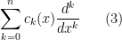
Clearly, for any polynomial 


and similarly the operator 
Inspired by this, if 
for all 


one can easily verify from several applications of the Leibniz rule that 


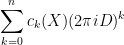
For instance, any constant coefficient linear differential operators 
however there are many Fourier multiplier operators that are not of this form, such as fractional derivative operators 


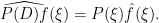
We observe that the maps 


and

for any 


for 
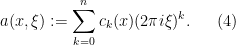
In the field of PDE and ODE, it is also very common to study variable coefficient linear differential operators
where the 

and so it is natural to interpret this operator as a combination 


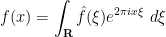
Indeed, from the Fourier inversion formula
for any
and hence on multiplying by 
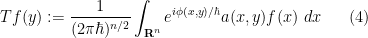
Inspired by this, we can introduce the Kohn-Nirenberg quantisation by defining the operator 
whenever
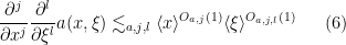
for all 


 are two functions obeying
  for all
  . (Hint: apply
  to a suitable truncation of a plane wave
  and then take limits.)
In principle, the quantisations 

in general. Fundamentally, this is due to the fact that pointwise multiplication of symbols is a commutative operation, whereas the composition of operators such as
![\displaystyle [A,B] := AB - BA](https://s0.wp.com/latex.php?latex=%5Cdisplaystyle++%5BA%2CB%5D+%3A%3D+AB+-+BA&bg=ffffff&fg=000000&s=0&c=20201002)
of two operators 
![\displaystyle [X,D] = -\frac{1}{2\pi i} \neq 0.](https://s0.wp.com/latex.php?latex=%5Cdisplaystyle++%5BX%2CD%5D+%3D+-%5Cfrac%7B1%7D%7B2%5Cpi+i%7D+%5Cneq+0.&bg=ffffff&fg=000000&s=0&c=20201002)
(In the language of Lie groups and Lie algebras, this tells us that
Exercise 2 (Heisenberg uncertainty principle) For any
and
, show that
(Hint: evaluate the expression
in two different ways and apply the Cauchy-Schwarz inequality.) Informally, this exercise asserts that the spatial uncertainty
and the frequency uncertainty
of a function obey the Heisenberg uncertainty relation
.

Nevertheless, one still has the correspondence principle, which asserts that in certain regimes (which, with our choice of normalisations, corresponds to the high-frequency regime), quantum mechanics continues to behave like a commutative theory, and one can sometimes proceed as if the operators

where the error between the left and right-hand sides is of “lower order” and can in fact enjoys a useful asymptotic expansion. As a first approximation to this calculus, one can think of functions 


Unfortunately the uncertainty principle (or the non-commutativity of 

To complement the pseudodifferential calculus we have the basic Calderón-Vaillancourt theorem, which asserts that pseudodifferential operators of order zero are Calderón-Zygmund operators and thus bounded on 

Pseudodifferential operators (especially when generalised to higher dimensions 
This set of notes is only the briefest introduction to the theory of pseudodifferential operators. Many texts are available that cover the theory in more detail, for instance this text of Taylor.
Lars Hörmander, who made fundamental contributions to all areas of partial differential equations, but particularly in developing the analysis of variable-coefficient linear PDE, died last Sunday, aged 81.
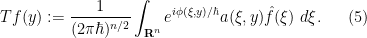
I unfortunately never met Hörmander personally, but of course I encountered his work all the time while working in PDE. One of his major contributions to the subject was to systematically develop the calculus of Fourier integral operators (FIOs), which are a substantial generalisation of pseudodifferential operators and which can be used to (approximately) solve linear partial differential equations, or to transform such equations into a more convenient form. Roughly speaking, Fourier integral operators are to linear PDE as canonical transformations are to Hamiltonian mechanics (and one can in fact view FIOs as a quantisation of a canonical transformation). They are a large class of transformations, for instance the Fourier transform, pseudodifferential operators, and smooth changes of the spatial variable are all examples of FIOs, and (as long as certain singular situations are avoided) the composition of two FIOs is again an FIO.
The full theory of FIOs is quite extensive, occupying the entire final volume of Hormander’s famous four-volume series “The Analysis of Linear Partial Differential Operators”. I am certainly not going to try to attempt to summarise it here, but I thought I would try to motivate how these operators arise when trying to transform functions. For simplicity we will work with functions 

A function 


where 


For instance, for the gaussian wave packet (1), one has

and so we see that 
However, there is a third (but less rigorous) way to view a function 


If functions in 
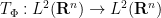
Now we turn to operators that alter the support of a phase space distribution, rather than the amplitude; we will focus on unitary operators to emphasise the amplitude preservation aspect. These will eventually be key examples of Fourier integral operators. A physical translation 


Based on these examples, one may hope that given any diffeomorphism 


and thus 

The formalisation of this fact in the theory of Fourier integral operators is known as Egorov’s theorem, due to Yu Egorov (and not to be confused with the more widely known theorem of Dmitri Egorov in measure theory).
Applying commutators, we conclude the approximate conjugacy relationship
![\displaystyle \frac{1}{i\hbar} [(a \circ \Phi)(X,D), (b \circ \Phi)(X,D)] \approx T_\Phi^{-1} \frac{1}{i\hbar} [a(X,D), b(X,D)] T_\Phi.](https://s0.wp.com/latex.php?latex=%5Cdisplaystyle++%5Cfrac%7B1%7D%7Bi%5Chbar%7D+%5B%28a+%5Ccirc+%5CPhi%29%28X%2CD%29%2C+%28b+%5Ccirc+%5CPhi%29%28X%2CD%29%5D+%5Capprox+T_%5CPhi%5E%7B-1%7D+%5Cfrac%7B1%7D%7Bi%5Chbar%7D+%5Ba%28X%2CD%29%2C+b%28X%2CD%29%5D+T_%5CPhi.&bg=ffffff&fg=000000&s=0&c=20201002)
Now, the pseudodifferential calculus (as discussed in this previous post) tells us (heuristically, at least) that
![\displaystyle \frac{1}{i\hbar} [a(X,D), b(X,D)] \approx \{ a, b \}(X,D)](https://s0.wp.com/latex.php?latex=%5Cdisplaystyle++%5Cfrac%7B1%7D%7Bi%5Chbar%7D+%5Ba%28X%2CD%29%2C+b%28X%2CD%29%5D+%5Capprox+%5C%7B+a%2C+b+%5C%7D%28X%2CD%29&bg=ffffff&fg=000000&s=0&c=20201002)
and
![\displaystyle \frac{1}{i\hbar} [(a \circ \Phi)(X,D), (b \circ \Phi)(X,D)] \approx \{ a \circ \Phi, b \circ \Phi \}(X,D)](https://s0.wp.com/latex.php?latex=%5Cdisplaystyle++%5Cfrac%7B1%7D%7Bi%5Chbar%7D+%5B%28a+%5Ccirc+%5CPhi%29%28X%2CD%29%2C+%28b+%5Ccirc+%5CPhi%29%28X%2CD%29%5D+%5Capprox+%5C%7B+a+%5Ccirc+%5CPhi%2C+b+%5Ccirc+%5CPhi+%5C%7D%28X%2CD%29&bg=ffffff&fg=000000&s=0&c=20201002)
where 

thus
Now suppose that 


for some smooth functions 


for 

for some smooth potential function 

so that 

A reasonable candidate for an operator associated to
for some smooth amplitude function 


Of course, it may be the case that 

This class of FIOs covers many important cases; for instance, the translation, modulation, and dilation operators considered earlier can be written in this form after some Fourier analysis. Another typical example is the half-wave propagator 

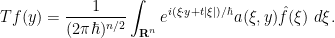
This corresponds to the phase space transformation 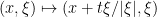


In some cases, the canonical relation

Recent Comments