Inverting the Schur complement, and large-dimensional Gelfand-Tsetlin patterns

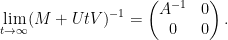
Suppose we have an matrix that is expressed in block-matrix form as

where is an matrix, is an matrix, is an matrix, and is a matrix for some . If is invertible, we can use the technique of Schur complementation to express the inverse of (if it exists) in terms of the inverse of , and the other components of course. Indeed, to solve the equation

where are column vectors and are column vectors, we can expand this out as a system

Using the invertibility of , we can write the first equation as

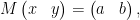
and substituting this into the second equation yields

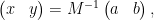
and thus (assuming that is invertible)

and then inserting this back into (1) gives

Comparing this with

we have managed to express the inverse of as

One can consider the inverse problem: given the inverse of , does one have a nice formula for the inverse of the minor ? Trying to recover this directly from (2) looks somewhat messy. However, one can proceed as follows. Let denote the matrix

(with the identity matrix), and let be its transpose:

Then for any scalar (which we identify with times the identity matrix), one has

and hence by (2)

noting that the inverses here will exist for large enough. Taking limits as , we conclude that

On the other hand, by the Woodbury matrix identity (discussed in this previous blog post), we have

and hence on taking limits and comparing with the preceding identity, one has

This achieves the aim of expressing the inverse of the minor in terms of the inverse of the full matrix. Taking traces and rearranging, we conclude in particular that

In the case, this can be simplified to

where is the basis column vector.

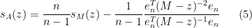
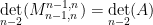
We can apply this identity to understand how the spectrum of an random matrix relates to that of its top left minor . Subtracting any complex multiple of the identity from (and hence from ), we can relate the Stieltjes transform of with the Stieltjes transform of :

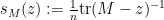
At this point we begin to proceed informally. Assume for sake of argument that the random matrix is Hermitian, with distribution that is invariant under conjugation by the unitary group ; for instance, could be drawn from the Gaussian Unitary Ensemble (GUE), or alternatively could be of the form for some real diagonal matrix and a unitary matrix drawn randomly from using Haar measure. To fix normalisations we will assume that the eigenvalues of are typically of size . Then is also Hermitian and -invariant. Furthermore, the law of will be the same as the law of , where is now drawn uniformly from the unit sphere (independently of ). Diagonalising into eigenvalues and eigenvectors , we have

One can think of as a random (complex) Gaussian vector, divided by the magnitude of that vector (which, by the Chernoff inequality, will concentrate to ). Thus the coefficients with respect to the orthonormal basis can be thought of as independent (complex) Gaussian vectors, divided by that magnitude. Using this and the Chernoff inequality again, we see (for distance away from the real axis at least) that one has the concentration of measure

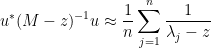
and thus

(that is to say, the diagonal entries of are roughly constant). Similarly we have

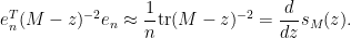
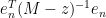
Inserting this into (5) and discarding terms of size , we thus conclude the approximate relationship

This can be viewed as a difference equation for the Stieltjes transform of top left minors of . Iterating this equation, and formally replacing the difference equation by a differential equation in the large limit, we see that when is large and for some , one expects the top left minor of to have Stieltjes transform

where solves the Burgers-type equation

with initial data .

Example 1 If is a constant multiple of the identity, then . One checks that is a steady state solution to (7), which is unsurprising given that all minors of are also times the identity.

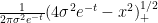
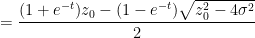
Example 2 If is GUE normalised so that each entry has variance , then by the semi-circular law (see previous notes) one has (using an appropriate branch of the square root). One can then verify the self-similar solution

to (7), which is consistent with the fact that a top minor of also has the law of GUE, with each entry having variance when .

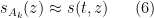
One can justify the approximation (6) given a sufficiently good well-posedness theory for the equation (7). We will not do so here, but will note that (as with the classical inviscid Burgers equation) the equation can be solved exactly (formally, at least) by the method of characteristics. For any initial position , we consider the characteristic flow formed by solving the ODE

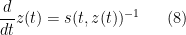
with initial data , ignoring for this discussion the problems of existence and uniqueness. Then from the chain rule, the equation (7) implies that

and thus . Inserting this back into (8) we see that

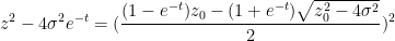
and thus (7) may be solved implicitly via the equation

for all and .

Remark 3 In practice, the equation (9) may stop working when crosses the real axis, as (7) does not necessarily hold in this region. It is a cute exercise (ultimately coming from the Cauchy-Schwarz inequality) to show that this crossing always happens, for instance if has positive imaginary part then necessarily has negative or zero imaginary part.

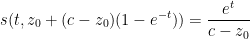
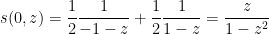
Example 4 Suppose we have as in Example 1. Then (9) becomes

for any , which after making the change of variables becomes

as in Example 1.

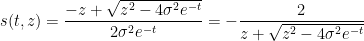
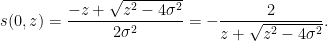
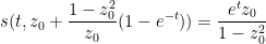
Example 5 Suppose we have

as in Example 2. Then (9) becomes

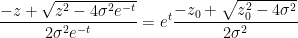
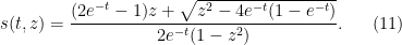
If we write

one can calculate that

and hence

which gives

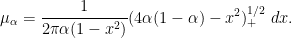
One can recover the spectral measure from the Stieltjes transform as the weak limit of as ; we write this informally as

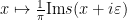
In this informal notation, we have for instance that

which can be interpreted as the fact that the Cauchy distributions converge weakly to the Dirac mass at as . Similarly, the spectral measure associated to (10) is the semicircular measure .

If we let be the spectral measure associated to , then the curve from to the space of measures is the high-dimensional limit of a Gelfand-Tsetlin pattern (discussed in this previous post), if the pattern is randomly generated amongst all matrices with spectrum asymptotic to as . For instance, if , then the curve is , corresponding to a pattern that is entirely filled with ‘s. If instead is a semicircular distribution, then the pattern is

thus at height from the top, the pattern is semicircular on the interval . The interlacing property of Gelfand-Tsetlin patterns translates to the claim that (resp. ) is non-decreasing (resp. non-increasing) in for any fixed . In principle one should be able to establish these monotonicity claims directly from the PDE (7) or from the implicit solution (9), but it was not clear to me how to do so.

An interesting example of such a limiting Gelfand-Tsetlin pattern occurs when , which corresponds to being , where is an orthogonal projection to a random -dimensional subspace of . Here we have

and so (9) in this case becomes

A tedious calculation then gives the solution

For , there are simple poles at , and the associated measure is

This reflects the interlacing property, which forces of the eigenvalues of the minor to be equal to (resp. ). For , the poles disappear and one just has

For , one has an inverse semicircle distribution

There is presumably a direct geometric explanation of this fact (basically describing the singular values of the product of two random orthogonal projections to half-dimensional subspaces of ), but I do not know of one off-hand.

The evolution of can also be understood using the -transform and -transform from free probability. Formally, letlet be the inverse of , thus

for all , and then define the -transform

The equation (9) may be rewritten as

and hence

or equivalently

See these previous notes for a discussion of free probability topics such as the -transform.

Example 6 If then the transform is .

Example 7 If is given by (10), then the transform is

Example 8 If is given by (11), then the transform is

This simple relationship (12) is essentially due to Nica and Speicher (thanks to Dima Shylakhtenko for this reference). It has the remarkable consequence that when is the reciprocal of a natural number , then is the free arithmetic mean of copies of , that is to say is the free convolution of copies of , pushed forward by the map . In terms of random matrices, this is asserting that the top minor of a random matrix has spectral measure approximately equal to that of an arithmetic mean of independent copies of , so that the process of taking top left minors is in some sense a continuous analogue of the process of taking freely independent arithmetic means. There ought to be a geometric proof of this assertion, but I do not know of one. In the limit (or ), the -transform becomes linear and the spectral measure becomes semicircular, which is of course consistent with the free central limit theorem.

In a similar vein, if one defines the function

and inverts it to obtain a function with

for all , then the -transform is defined by

Writing

for any , , we have

and so (9) becomes

which simplifies to

replacing by we obtain

and thus

and hence

One can compute to be the -transform of the measure ; from the link between -transforms and free products (see e.g. these notes of Guionnet), we conclude that is the free product of and . This is consistent with the random matrix theory interpretation, since is also the spectral measure of , where is the orthogonal projection to the span of the first basis elements, so in particular has spectral measure . If is unitarily invariant then (by a fundamental result of Voiculescu) it is asymptotically freely independent of , so the spectral measure of is asymptotically the free product of that of and of .

Dodgson condensation from Schur complementation

The determinant of an matrix (with coefficients in an arbitrary field) obey many useful identities, starting of course with the fundamental multiplicativity for matrices . This multiplicativity can in turn be used to establish many further identities; in particular, as shown in this previous post, it implies the Schur determinant identity

whenever is an invertible matrix, is an matrix, is a matrix, and is a matrix. The matrix is known as the Schur complement of the block .

I only recently discovered that this identity in turn immediately implies what I always found to be a somewhat curious identity, namely the Dodgson condensation identity (also known as the Desnanot-Jacobi identity)

for any and matrix , where denotes the matrix formed from by removing the row and column, and similarly denotes the matrix formed from by removing the and rows and and columns. Thus for instance when we obtain

for any scalars . (Charles Dodgson, better known by his pen name Lewis Caroll, is of course also known for writing “Alice in Wonderland” and “Through the Looking Glass“.)

The derivation is not new; it is for instance noted explicitly in this paper of Brualdi and Schneider, though I do not know if this is the earliest place in the literature where it can be found. (EDIT: Apoorva Khare has pointed out to me that the original arguments of Dodgson can be interpreted as implicitly following this derivation.) I thought it is worth presenting the short derivation here, though.

Firstly, by swapping the first and rows, and similarly for the columns, it is easy to see that the Dodgson condensation identity is equivalent to the variant

Now write

where is an matrix, are column vectors, are row vectors, and are scalars. If is invertible, we may apply the Schur determinant identity repeatedly to conclude that

and the claim (2) then follows by a brief calculation (and the explicit form of the determinant). To remove the requirement that be invertible, one can use a limiting argument, noting that one can work without loss of generality in an algebraically closed field, and in such a field, the set of invertible matrices is dense in the Zariski topology. (In the case when the scalars are reals or complexes, one can just use density in the ordinary topology instead if desired.)

The same argument gives the more general determinant identity of Sylvester

whenever , is a -element subset of , and denotes the matrix formed from by removing the rows associated to and the columns associated to . (The Dodgson condensation identity is basically the case of this identity.)

A closely related proof of (2) proceeds by elementary row and column operations. Observe that if one adds some multiple of one of the first rows of to one of the last two rows of , then the left and right sides of (2) do not change. If the minor is invertible, this allows one to reduce to the case where the components of the matrix vanish. Similarly, using elementary column operations instead of row operations we may assume that vanish. All matrices involved are now block-diagonal and the identity follows from a routine computation.

The latter approach can also prove the cute identity

for any , any column vectors , and any matrix , which can for instance be found in page 7 of this text of Karlin. Observe that both sides of this identity are unchanged if one adds some multiple of any column of to one of ; for generic , this allows one to reduce to have only the first two entries allowed to be non-zero, at which point the determinants split into and determinants and we can reduce to the case (eliminating the role of ). One can now either proceed by a direct computation, or by observing that the left-hand side is quartilinear in and antisymmetric in and which forces it to be a scalar multiple of , at which point one can test the identity at a single point (e.g. and for the standard basis ) to conclude the argument. (One can also derive this identity from the Sylvester determinant identity but I think the calculations are a little messier if one goes by that route. Conversely, one can recover the Dodgson condensation identity from Karlin’s identity by setting , (for instance) and then permuting some rows and columns.)

Matrix identities as derivatives of determinant identities

The determinant of a square matrix obeys a large number of important identities, the most basic of which is the multiplicativity property

whenever are square matrices of the same dimension. This identity then generates many other important identities. For instance, if is an matrix and is an matrix, then by applying the previous identity to equate the determinants of and (where we will adopt the convention that denotes an identity matrix of whatever dimension is needed to make sense of the expressions being computed, and similarly for ) we obtain the Weinstein-Aronszajn determinant identity

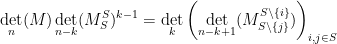
This identity, which converts an determinant into an determinant, is very useful in random matrix theory (a point emphasised in particular by Deift), particularly in regimes in which is much smaller than .

Another identity generated from (1) arises when trying to compute the determinant of a block matrix

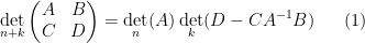
where is an matrix, is an matrix, is an matrix, and is an matrix. If is invertible, then we can manipulate this matrix via block Gaussian elimination as

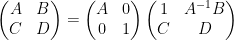
and on taking determinants using (1) we obtain the Schur determinant identity

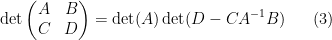
relating the determinant of a block-diagonal matrix with the determinant of the Schur complement of the upper left block . This identity can be viewed as the correct way to generalise the determinant formula

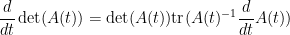
It is also possible to use determinant identities to deduce other matrix identities that do not involve the determinant, by the technique of matrix differentiation (or equivalently, matrix linearisation). The key observation is that near the identity, the determinant behaves like the trace, or more precisely one has

for any bounded square matrix and infinitesimal . (If one is uncomfortable with infinitesimals, one can interpret this sort of identity as an asymptotic as .) Combining this with (1) we see that for square matrices of the same dimension with invertible and invertible, one has

for infinitesimal . To put it another way, if is a square matrix that depends in a differentiable fashion on a real parameter , then we have the Jacobi formula

whenever is invertible. (Note that if one combines this identity with cofactor expansion, one recovers Cramer’s rule.)

Let us see some examples of this differentiation method. If we take the Weinstein-Aronszajn identity (2) and multiply one of the rectangular matrices by an infinitesimal , we obtain

applying (4) and extracting the linear term in (or equivalently, differentiating at and then setting ) we conclude the cyclic property of trace:

To manipulate derivatives and inverses, we begin with the Neumann series approximation

for bounded square and infinitesimal , which then leads to the more general approximation

for square matrices of the same dimension with bounded. To put it another way, we have

whenever depends in a differentiable manner on and is invertible.

We can then differentiate (or linearise) the Schur identity (3) in a number of ways. For instance, if we replace the lower block by for some test matrix , then by (4), the left-hand side of (3) becomes (assuming the invertibility of the block matrix)

while the right-hand side becomes

extracting the linear term in , we conclude that

As was an arbitrary matrix, we conclude from duality that the lower right block of is given by the inverse of the Schur complement:

One can also compute the other components of this inverse in terms of the Schur complement by a similar method (although the formulae become more complicated). As a variant of this method, we can perturb the block matrix in (3) by an infinitesimal multiple of the identity matrix giving

By (4), the left-hand side is

From (5), we have

and so from (4) the right-hand side of (6) is

extracting the linear component in , we conclude the identity

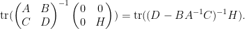
which relates the trace of the inverse of a block matrix, with the trace of the inverse of one of its blocks. This particular identity turns out to be useful in random matrix theory; I hope to elaborate on this in a later post.

As a final example of this method, we can analyse low rank perturbations of a large () matrix , where is an matrix and is an matrix for some . (This type of situation is also common in random matrix theory, for instance it arose in this previous paper of mine on outliers to the circular law.) If is invertible, then from (1) and (2) one has the matrix determinant lemma

if one then perturbs by an infinitesimal matrix , we have

Extracting the linear component in as before, one soon arrives at

assuming that and are both invertible; as is arbitrary, we conclude (after using the cyclic property of trace) the Sherman-Morrison formula

for the inverse of a low rank perturbation of a matrix . While this identity can be easily verified by direct algebraic computation, it is somewhat difficult to discover this identity by such algebraic manipulation; thus we see that the “determinant first” approach to matrix identities can make it easier to find appropriate matrix identities (particularly those involving traces and/or inverses), even if the identities one is ultimately interested in do not involve determinants. (As differentiation typically makes an identity lengthier, but also more “linear” or “additive”, the determinant identity tends to be shorter (albeit more nonlinear and more multiplicative) than the differentiated identity, and can thus be slightly easier to derive.)

Exercise 1 Use the “determinant first” approach to derive the Woodbury matrix identity (also known as the binomial inverse theorem)

where is an matrix, is an matrix, is an matrix, and is an matrix, assuming that , and are all invertible.

Exercise 2 Let be invertible matrices. Establish the identity

and differentiate this in to deduce the identity

(assuming that all inverses exist) and thence

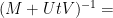
Rotating by then gives

which is useful for inverting a matrix that has been split into a self-adjoint component and a skew-adjoint component .