Multiple recurrence and convergence results associated to F_p^omega-actions

Vitaly Bergelson, Tamar Ziegler, and I have just uploaded to the arXiv our joint paper “Multiple recurrence and convergence results associated to -actions“. This paper is primarily concerned with limit formulae in the theory of multiple recurrence in ergodic theory. Perhaps the most basic formula of this type is the mean ergodic theorem, which (among other things) asserts that if is a measure-preserving -system (which, in this post, means that is a probability space and is measure-preserving and invertible, thus giving an action of the integers), and are functions, and is ergodic (which means that contains no -invariant functions other than the constants (up to almost everywhere equivalence, of course)), then the average

converges as to the expression

see e.g. this previous blog post. Informally, one can interpret this limit formula as an equidistribution result: if is drawn at random from (using the probability measure ), and is drawn at random from for some large , then the pair becomes uniformly distributed in the product space (using product measure ) in the limit as .

If we allow to be non-ergodic, then we still have a limit formula, but it is a bit more complicated. Let be the -invariant measurable sets in ; the -system can then be viewed as a factor of the original system , which is equivalent (in the sense of measure-preserving systems) to a trivial system (known as the invariant factor) in which the shift is trivial. There is then a projection map to the invariant factor which is a factor map, and the average (1) converges in the limit to the expression

where is the pushforward map associated to the map ; see e.g. this previous blog post. We can interpret this as an equidistribution result. If is a pair as before, then we no longer expect complete equidistribution in in the non-ergodic, because there are now non-trivial constraints relating with ; indeed, for any -invariant function , we have the constraint ; putting all these constraints together we see that (for almost every , at least). The limit (2) can be viewed as an assertion that this constraint are in some sense the “only” constraints between and , and that the pair is uniformly distributed relative to these constraints.

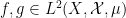
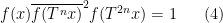
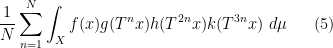
Limit formulae are known for multiple ergodic averages as well, although the statement becomes more complicated. For instance, consider the expression

for three functions ; this is analogous to the combinatorial task of counting length three progressions in various sets. For simplicity we assume the system to be ergodic. Naively one might expect this limit to then converge to

which would roughly speaking correspond to an assertion that the triplet is asymptotically equidistributed in . However, even in the ergodic case there can be additional constraints on this triplet that cannot be seen at the level of the individual pairs , . The key obstruction here is that of eigenfunctions of the shift , that is to say non-trivial functions that obey the eigenfunction equation almost everywhere for some constant (or -invariant) . Each such eigenfunction generates a constraint

tying together , , and . However, it turns out that these are in some sense the only constraints on that are relevant for the limit (3). More precisely, if one sets to be the sub-algebra of generated by the eigenfunctions of , then it turns out that the factor is isomorphic to a shift system known as the Kronecker factor, for some compact abelian group and some (irrational) shift ; the factor map pushes eigenfunctions forward to (affine) characters on . It is then known that the limit of (3) is

where is the closed subgroup

and is the Haar probability measure on ; see this previous blog post. The equation defining corresponds to the constraint (4) mentioned earlier. Among other things, this limit formula implies Roth’s theorem, which in the context of ergodic theory is the assertion that the limit (or at least the limit inferior) of (3) is positive when is non-negative and not identically vanishing.

If one considers a quadruple average

(analogous to counting length four progressions) then the situation becomes more complicated still, even in the ergodic case. In addition to the (linear) eigenfunctions that already showed up in the computation of the triple average (3), a new type of constraint also arises from quadratic eigenfunctions , which obey an eigenfunction equation in which is no longer constant, but is now a linear eigenfunction. For such functions, behaves quadratically in , and one can compute the existence of a constraint

between , , , and that is not detected at the triple average level. As it turns out, this is not the only type of constraint relevant for (5); there is a more general class of constraint involving two-step nilsystems which we will not detail here, but see e.g. this previous blog post for more discussion. Nevertheless there is still a similar limit formula to previous examples, involving a special factor which turns out to be an inverse limit of two-step nilsystems; this limit theorem can be extracted from the structural theory in this paper of Host and Kra combined with a limit formula for nilsystems obtained by Lesigne, but will not be reproduced here. The pattern continues to higher averages (and higher step nilsystems); this was first done explicitly by Ziegler, and can also in principle be extracted from the structural theory of Host-Kra combined with nilsystem equidistribution results of Leibman. These sorts of limit formulae can lead to various recurrence results refining Roth’s theorem in various ways; see this paper of Bergelson, Host, and Kra for some examples of this.

The above discussion was concerned with -systems, but one can adapt much of the theory to measure-preserving -systems for other discrete countable abelian groups , in which one now has a family of shifts indexed by rather than a single shift, obeying the compatibility relation . The role of the intervals in this more general setting is replaced by that of Folner sequences. For arbitrary countable abelian , the theory for double averages (1) and triple limits (3) is essentially identical to the -system case. But when one turns to quadruple and higher limits, the situation becomes more complicated (and, for arbitrary , still not fully understood). However one model case which is now well understood is the finite field case when is an infinite-dimensional vector space over a finite field (with the finite subspaces then being a good choice for the Folner sequence). Here, the analogue of the structural theory of Host and Kra was worked out by Vitaly, Tamar, and myself in these previous papers (treating the high characteristic and low characteristic cases respectively). In the finite field setting, it turns out that nilsystems no longer appear, and one only needs to deal with linear, quadratic, and higher order eigenfunctions (known collectively as phase polynomials). It is then natural to look for a limit formula that asserts, roughly speaking, that if is drawn at random from a -system and drawn randomly from a large subspace of , then the only constraints between are those that arise from phase polynomials. The main theorem of this paper is to establish this limit formula (which, again, is a little complicated to state explicitly and will not be done here). In particular, we establish for the first time that the limit actually exists (a result which, for -systems, was one of the main results of this paper of Host and Kra).

As a consequence, we can recover finite field analogues of most of the results of Bergelson-Host-Kra, though interestingly some of the counterexamples demonstrating sharpness of their results for -systems (based on Behrend set constructions) do not seem to be present in the finite field setting (cf. this previous blog post on the cap set problem). In particular, we are able to largely settle the question of when one has a Khintchine-type theorem that asserts that for any measurable set in an ergodic -system and any , one has

for a syndetic set of , where are distinct residue classes. It turns out that Khintchine-type theorems always hold for (and for ergodicity is not required), and for it holds whenever form a parallelogram, but not otherwise (though the counterexample here was such a painful computation that we ended up removing it from the paper, and may end up putting it online somewhere instead), and for larger we could show that the Khintchine property failed for generic choices of , though the problem of determining exactly the tuples for which the Khintchine property failed looked to be rather messy and we did not completely settle it.

Multiple recurrence in quasirandom groups

I’ve just uploaded to the arXiv my joint paper with Vitaly Bergelson, “Multiple recurrence in quasirandom groups“, which is submitted to Geom. Func. Anal.. This paper builds upon a paper of Gowers in which he introduced the concept of a quasirandom group, and established some mixing (or recurrence) properties of such groups. A -quasirandom group is a finite group with no non-trivial unitary representations of dimension at most . We will informally refer to a “quasirandom group” as a -quasirandom group with the quasirandomness parameter large (more formally, one can work with a sequence of -quasirandom groups with going to infinity). A typical example of a quasirandom group is where is a large prime. Quasirandom groups are discussed in depth in this blog post. One of the key properties of quasirandom groups established in Gowers’ paper is the following “weak mixing” property: if are subsets of , then for “almost all” , one has

where denotes the density of in . Here, we use to informally represent an estimate of the form (where is a quantity that goes to zero when the quasirandomness parameter goes to infinity), and “almost all ” denotes “for all in a subset of of density “. As a corollary, if have positive density in (by which we mean that is bounded away from zero, uniformly in the quasirandomness parameter , and similarly for ), then (if the quasirandomness parameter is sufficiently large) we can find elements such that , , . In fact we can find approximately such pairs . To put it another way: if we choose uniformly and independently at random from , then the events , , are approximately independent (thus the random variable resembles a uniformly distributed random variable on in some weak sense). One can also express this mixing property in integral form as

for any bounded functions . (Of course, with being finite, one could replace the integrals here by finite averages if desired.) Or in probabilistic language, we have

where are drawn uniformly and independently at random from .

As observed in Gowers’ paper, one can iterate this observation to find “parallelopipeds” of any given dimension in dense subsets of . For instance, applying (1) with replaced by , , and one can assert (after some relabeling) that for chosen uniformly and independently at random from , the events , , , , , , are approximately independent whenever are dense subsets of ; thus the tuple resebles a uniformly distributed random variable in in some weak sense.

However, there are other tuples for which the above iteration argument does not seem to apply. One of the simplest tuples in this vein is the tuple in , when are drawn uniformly at random from a quasirandom group . Here, one does not expect the tuple to behave as if it were uniformly distributed in , because there is an obvious constraint connecting the last two components of this tuple: they must lie in the same conjugacy class! In particular, if is a subset of that is the union of conjugacy classes, then the events , are perfectly correlated, so that is equal to rather than . Our main result, though, is that in a quasirandom group, this is (approximately) the only constraint on the tuple. More precisely, we have

Theorem 1 Let be a -quasirandom group, and let be drawn uniformly at random from . Then for any , we have

where goes to zero as , are drawn uniformly and independently at random from , and is drawn uniformly at random from the conjugates of for each fixed choice of .

This is the probabilistic formulation of the above theorem; one can also phrase the theorem in other formulations (such as an integral formulation), and this is detailed in the paper. This theorem leads to a number of recurrence results; for instance, as a corollary of this result, we have

for almost all , and any dense subsets of ; the lower and upper bounds are sharp, with the lower bound being attained when is randomly distributed, and the upper bound when is conjugation-invariant.

To me, the more interesting thing here is not the result itself, but how it is proven. Vitaly and I were not able to find a purely finitary way to establish this mixing theorem. Instead, we had to first use the machinery of ultraproducts (as discussed in this previous post) to convert the finitary statement about a quasirandom group to an infinitary statement about a type of infinite group which we call an ultra quasirandom group (basically, an ultraproduct of increasingly quasirandom finite groups). This is analogous to how the Furstenberg correspondence principle is used to convert a finitary combinatorial problem into an infinitary ergodic theory problem.

Ultra quasirandom groups come equipped with a finite, countably additive measure known as Loeb measure , which is very analogous to the Haar measure of a compact group, except that in the case of ultra quasirandom groups one does not quite have a topological structure that would give compactness. Instead, one has a slightly weaker structure known as a -topology, which is like a topology except that open sets are only closed under countable unions rather than arbitrary ones. There are some interesting measure-theoretic and topological issues regarding the distinction between topologies and -topologies (and between Haar measure and Loeb measure), but for this post it is perhaps best to gloss over these issues and pretend that ultra quasirandom groups come with a Haar measure. One can then recast Theorem 1 as a mixing theorem for the left and right actions of the ultra approximate group on itself, which roughly speaking is the assertion that

for “almost all” , if are bounded measurable functions on , with having zero mean on all conjugacy classes of , where are the left and right translation operators

To establish this mixing theorem, we use the machinery of idempotent ultrafilters, which is a particularly useful tool for understanding the ergodic theory of actions of countable groups that need not be amenable; in the non-amenable setting the classical ergodic averages do not make much sense, but ultrafilter-based averages are still available. To oversimplify substantially, the idempotent ultrafilter arguments let one establish mixing estimates of the form (2) for “many” elements of an infinite-dimensional parallelopiped known as an IP system (provided that the actions of this IP system obey some technical mixing hypotheses, but let’s ignore that for sake of this discussion). The claim then follows by using the quasirandomness hypothesis to show that if the estimate (2) failed for a large set of , then this large set would then contain an IP system, contradicting the previous claim.

Idempotent ultrafilters are an extremely infinitary type of mathematical object (one has to use Zorn’s lemma no fewer than three times just to construct one of these objects!). So it is quite remarkable that they can be used to establish a finitary theorem such as Theorem 1, though as is often the case with such infinitary arguments, one gets absolutely no quantitative control whatsoever on the error terms appearing in that theorem. (It is also mildly amusing to note that our arguments involve the use of ultrafilters in two completely different ways: firstly in order to set up the ultraproduct that converts the finitary mixing problem to an infinitary one, and secondly to solve the infinitary mixing problem. Despite some superficial similarities, there appear to be no substantial commonalities between these two usages of ultrafilters.) There is already a fair amount of literature on using idempotent ultrafilter methods in infinitary ergodic theory, and perhaps by further development of ultraproduct correspondence principles, one can use such methods to obtain further finitary consequences (although the state of the art for idempotent ultrafilter ergodic theory has not advanced much beyond the analysis of two commuting shifts currently, which is the main reason why our arguments only handle the pattern and not more sophisticated patterns).

We also have some miscellaneous other results in the paper. It turns out that by using the triangle removal lemma from graph theory, one can obtain a recurrence result that asserts that whenever is a dense subset of a finite group (not necessarily quasirandom), then there are pairs such that all lie in . Using a hypergraph generalisation of the triangle removal lemma known as the hypergraph removal lemma, one can obtain more complicated versions of this statement; for instance, if is a dense subset of , then one can find triples such that all lie in . But the method is tailored to the specific types of patterns given here, and we do not have a general method for obtaining recurrence or mixing properties for arbitrary patterns of words in some finite alphabet such as .

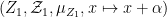
We also give some properties of a model example of an ultra quasirandom group, namely the ultraproduct of where is a sequence of primes going off to infinity. Thanks to the substantial recent progress (by Helfgott, Bourgain, Gamburd, Breuillard, and others) on understanding the expansion properties of the finite groups , we have a fair amount of knowledge on the ultraproduct as well; for instance any two elements of will almost surely generate a spectral gap. We don’t have any direct application of this particular ultra quasirandom group, but it might be interesting to study it further.

An inverse theorem for the uniformity seminorms associated with the action of F^infty_p

Vitaly Bergelson, Tamar Ziegler, and I have just uploaded to the arXiv our paper “An inverse theorem for the uniformity seminorms associated with the action of “. This paper establishes the ergodic inverse theorems that are needed in our other recent paper to establish the inverse conjecture for the Gowers norms over finite fields in high characteristic (and to establish a partial result in low characteristic), as follows:

Theorem. Let be a finite field of characteristic p.  Suppose that is a probability space with an ergodic measure-preserving action of .  Let be such that the Gowers-Host-Kra seminorm (defined in a previous post) is non-zero.

1. In the high-characteristic case , there exists a phase polynomial g of degree <k (as defined in the previous post) such that .
2. In general characteristic, there exists a phase polynomial of degree <C(k) for some C(k) depending only on k such that .

This theorem is closely analogous to a similar theorem of Host and Kra on ergodic actions of , in which the role of phase polynomials is played by functions that arise from nilsystem factors of X.  Indeed, our arguments rely heavily on the machinery of Host and Kra.

The paper is rather technical (60+ pages!) and difficult to describe in detail here, but I will try to sketch out (in very broad brush strokes) what the key steps in the proof of part 2 of the theorem are.  (Part 1 is similar but requires a more delicate analysis at various stages, keeping more careful track of the degrees of various polynomials.)

Some notes on “non-classical” polynomials in finite characteristic

Let be an integer.  The concept of a polynomial of one variable of degree (or ) can be defined in one of two equivalent ways:

• (Global definition) is a polynomial of degree iff it can be written in the form for some coefficients .
• (Local definition) is a polynomial of degree if it is k-times continuously differentiable and .

From single variable calculus we know that if P is a polynomial in the global sense, then it is a polynomial in the local sense; conversely, if P is a polynomial in the local sense, then from the Taylor series expansion

we see that P is a polynomial in the global sense. We make the trivial remark that we have no difficulty dividing by here, because the field is of characteristic zero.

The above equivalence carries over to higher dimensions:

• (Global definition) is a polynomial of degree iff it can be written in the form for some coefficients .
• (Local definition) is a polynomial of degree if it is k-times continuously differentiable and for all .

Again, it is not difficult to use several variable calculus to show that these two definitions of a polynomial are equivalent.

The purpose of this (somewhat technical) post here is to record some basic analogues of the above facts in finite characteristic, in which the underlying domain of the polynomial P is F or for some finite field F.  In the “classical” case when the range of P is also the field F, it is a well-known fact (which we reproduce here) that the local and global definitions of polynomial are equivalent.  But in the “non-classical” case, when P ranges in a more general group (and in particular in the unit circle ), the global definition needs to be corrected somewhat by adding some new monomials to the classical ones .  Once one does this, one can recover the equivalence between the local and global definitions.

(The results here are derived from forthcoming work with Vitaly Bergelson and Tamar Ziegler.)