A fundamental problem in analytic number theory is to understand the distribution of the prime numbers  . For technical reasons, it is convenient not to study the primes directly, but a proxy for the primes known as the von Mangoldt function
  , defined by setting
  to equal
  when
when  is a prime
  (or a power of that prime) and zero otherwise. The basic reason why the von Mangoldt function is useful is that it encodes the fundamental theorem of arithmetic (which in turn can be viewed as the defining property of the primes) very neatly via the identity

for every natural number .
The most important result in this subject is the prime number theorem, which asserts that the number of prime numbers less than a large number  is equal to
  :
:

Here, of course,  denotes a quantity that goes to zero as
  .
.
It is not hard to see (e.g. by summation by parts) that this is equivalent to the asymptotic
for the von Mangoldt function (the key point being that the squares, cubes, etc. of primes give a negligible contribution, so  is essentially the same quantity as
  ). Understanding the nature of the term is a very important problem, with the conjectured optimal decay rate of
  being equivalent to the Riemann hypothesis, but this will not be our concern here.
The prime number theorem has several important generalisations (for instance, there are analogues for other number fields such as the Chebotarev density theorem). One of the more elementary such generalisations is the prime number theorem in arithmetic progressions, which asserts that for fixed  and
and  with coprime to (thus
  ), the number of primes less than equal to mod is equal to
  , where
  is the Euler totient function:

(Of course, if is not coprime to , the number of primes less than equal to mod is  . The subscript in the
  and
and  notation denotes that the implied constants in that notation is allowed to depend on .) This is a more quantitative version of Dirichlet’s theorem, which asserts the weaker statement that the number of primes equal to mod is infinite. This theorem is important in many applications in analytic number theory, for instance in Vinogradov’s theorem that every sufficiently large odd number is the sum of three odd primes. (Imagine for instance if almost all of the primes were clustered in the residue class
  mod
mod  , rather than
  mod . Then almost all sums of three odd primes would be divisible by , leaving dangerously few sums left to cover the remaining two residue classes. Similarly for other moduli than . This does not fully rule out the possibility that Vinogradov’s theorem could still be true, but it does indicate why the prime number theorem in arithmetic progressions is a relevant tool in the proof of that theorem.)
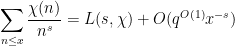
As before, one can rewrite the prime number theorem in arithmetic progressions in terms of the von Mangoldt function as the equivalent form
Philosophically, one of the main reasons why it is so hard to control the distribution of the primes is that we do not currently have too many tools with which one can rule out “conspiracies” between the primes, in which the primes (or the von Mangoldt function) decide to correlate with some structured object (and in particular, with a totally multiplicative function) which then visibly distorts the distribution of the primes. For instance, one could imagine a scenario in which the probability that a randomly chosen large integer is prime is not asymptotic to  (as is given by the prime number theorem), but instead to fluctuate depending on the phase of the complex number
  for some fixed real number
  , thus for instance the probability might be significantly less than
  when
when  is close to an integer, and significantly more than when is close to a half-integer. This would contradict the prime number theorem, and so this scenario would have to be somehow eradicated in the course of proving that theorem. In the language of Dirichlet series, this conspiracy is more commonly known as a zero of the Riemann zeta function at
  .
.
In the above scenario, the primality of a large integer was somehow sensitive to asymptotic or “Archimedean” information about , namely the approximate value of its logarithm. In modern terminology, this information reflects the local behaviour of at the infinite place  . There are also potential consipracies in which the primality of is sensitive to the local behaviour of at finite places, and in particular to the residue class of mod for some fixed modulus . For instance, given a Dirichlet character
  of modulus , i.e. a completely multiplicative function on the integers which is periodic of period (and vanishes on those integers not coprime to ), one could imagine a scenario in which the probability that a randomly chosen large integer is prime is large when
  is close to
  , and small when is close to
  , which would contradict the prime number theorem in arithmetic progressions. (Note the similarity between this scenario at and the previous scenario at ; in particular, observe that the functions
  and
and  are both totally multiplicative.) In the language of Dirichlet series, this conspiracy is more commonly known as a zero of the
  -function of
  at .
at .
An especially difficult scenario to eliminate is that of real characters, such as the Kronecker symbol  , in which numbers which are quadratic nonresidues mod are very likely to be prime, and quadratic residues mod are unlikely to be prime. Indeed, there is a scenario of this form – the Siegel zero scenario – which we are still not able to eradicate (without assuming powerful conjectures such as GRH), though fortunately Siegel zeroes are not quite strong enough to destroy the prime number theorem in arithmetic progressions.
It is difficult to prove that no conspiracy between the primes exist. However, it is not entirely impossible, because we have been able to exploit two important phenomena. The first is that there is often a “all or nothing dichotomy” (somewhat resembling the zero-one laws in probability) regarding conspiracies: in the asymptotic limit, the primes can either conspire totally (or more precisely, anti-conspire totally) with a multiplicative function, or fail to conspire at all, but there is no middle ground. (In the language of Dirichlet series, this is reflected in the fact that zeroes of a meromorphic function can have order , or order  (i.e. are not zeroes after all), but cannot have an intermediate order between and .) As a corollary of this fact, the prime numbers cannot conspire with two distinct multiplicative functions at once (by having a partial correlation with one and another partial correlation with another); thus one can use the existence of one conspiracy to exclude all the others. In other words, there is at most one conspiracy that can significantly distort the distribution of the primes. Unfortunately, this argument is ineffective, because it doesn’t give any control at all on what that conspiracy is, or even if it exists in the first place!
But now one can use the second important phenomenon, which is that because of symmetries, one type of conspiracy can lead to another. For instance, because the von Mangoldt function is real-valued rather than complex-valued, we have conjugation symmetry; if the primes correlate with, say, , then they must also correlate with  . (In the language of Dirichlet series, this reflects the fact that the zeta function and -functions enjoy symmetries with respect to reflection across the real axis (i.e. complex conjugation).) Combining this observation with the all-or-nothing dichotomy, we conclude that the primes cannot correlate with for any non-zero , which in fact leads directly to the prime number theorem (2), as we shall discuss below. Similarly, if the primes correlated with a Dirichlet character , then they would also correlate with the conjugate
  , which also is inconsistent with the all-or-nothing dichotomy, except in the exceptional case when is real – which essentially means that is a quadratic character. In this one case (which is the only scenario which comes close to threatening the truth of the prime number theorem in arithmetic progressions), the above tricks fail and one has to instead exploit the algebraic number theory properties of these characters instead, which has so far led to weaker results than in the non-real case.
As mentioned previously in passing, these phenomena are usually presented using the language of Dirichlet series and complex analysis. This is a very slick and powerful way to do things, but I would like here to present the elementary approach to the same topics, which is slightly weaker but which I find to also be very instructive. (However, I will not be too dogmatic about keeping things elementary, if this comes at the expense of obscuring the key ideas; in particular, I will rely on multiplicative Fourier analysis (both at and at finite places) as a substitute for complex analysis in order to expedite various parts of the argument. Also, the emphasis here will be more on heuristics and intuition than on rigour.)
The material here is closely related to the theory of pretentious characters developed by Granville and Soundararajan, as well as an earlier paper of Granville on elementary proofs of the prime number theorem in arithmetic progressions.
— 1. A heuristic elementary proof of the prime number theorem —
To motivate some of the later discussion, let us first give a highly non-rigorous heuristic elementary “proof” of the prime number theorem (2). Since we clearly have
one can view the prime number theorem as an assertion that the von Mangoldt function  “behaves like on the average”,

where we will be deliberately vague as to what the “ ” symbol means. (One can think of this symbol as denoting some sort of proximity in the weak topology or vague topology, after suitable normalisation.)
To see why one would expect (3) to be true, we take divisor sums of (3) to heuristically obtain

By (1), the left-hand side is  ; meanwhile, the right-hand side is the divisor function
  of , by definition. So we have a heuristic relationship between (3) and the informal approximation

In particular, we expect

The right-hand side of (6) can be approximated using the integral test as

(one can also use Stirling’s formula to obtain a similar asymptotic). As for the left-hand side, we write  and then make the substitution
  to obtain

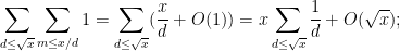
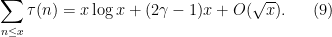
The right-hand side is the number of lattice points underneath the hyperbola  , and can be counted using the Dirichlet hyperbola method:

The third sum is equal to  . The second sum is equal to the first. The first sum can be computed as
meanwhile, from the integral test and the definition of Euler’s constant  one has

for any  ; combining all these estimates one obtains
Comparing this with (7) we do see that and are roughly equal “to top order” on average, thus giving some form of (5) and hence (4); if one could somehow invert the divisor sum operation, one could hope to get (3) and thus the prime number theorem.
(Looking at the next highest order terms in (7), (9), we see that we expect to in fact be slightly larger than on the average, and so should be slightly less than on the average. There is indeed a slight effect of this form; for instance, it is possible (using the prime number theorem) to prove

which should be compared with (8).)
One can partially translate the above discussion into the language of Dirichlet series, by transforming various arithmetical functions  to their associated Dirichlet series

ignoring for now the issue of convergence of this series. By definition, the constant function transforms to the Riemann zeta function  . Taking derivatives in
  , we see (formally, at least) that if has Dirichlet series
  , then
  has Dirichlet series
  ; thus, for instance, has Dirichlet series
  .
.
Most importantly, though, if  have Dirichlet series
  respectively, then their Dirichlet convolution
 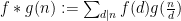 has Dirichlet series
  ; this is closely related to the well-known ability of the Fourier transform to convert convolutions to pointwise multiplication. Thus, for instance, has Dirichlet series
  . Also, from (1) and the preceding discussion, we see that has Dirichlet series
  (formally, at least). This already suggests that the von Mangoldt function will be sensitive to the zeroes of the zeta function.
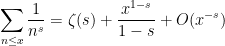
An integral test computation closely related to (8) gives the asymptotic

for close to one (and  , to avoid issues of convergence). This implies that the Dirichlet series for has asymptotic

thus giving support to (3); similarly, the Dirichlet series for and have asymptotic

and
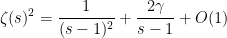
which gives support to (5) (and is also consistent with (7), (9)).
Remark 1 One can connect the properties of Dirichlet series more rigorously to asymptotics of partial sums  by means of various transforms in Fourier analysis and complex analysis, in particular contour integration or the Hilbert transform, but this becomes somewhat technical and we will not do so here. I will remark, though, that asymptotics of for close to are not enough, by themselves, to get really precise asymptotics for the sharply truncated partial sums , for reasons related to the uncertainty principle; in order to control such sums one also needs to understand the behaviour of
  far away from
  , and in particular for
  for large real . On the other hand, the asymptotics for for near are just about all one needs to control smoothly truncated partial sums such as
  for suitable cutoff functions
  . Also, while Dirichlet series are very powerful tools, particularly with regards to understanding Dirichlet convolution identities, and controlling everything in terms of the zeroes and poles of such series, they do have the drawback that they do not easily encode such fundamental “physical space” facts as the pointwise inequalities
  and
and  , which are also an important aspect of the theory.
— 2. Almost primes —
One can hope to make the above heuristics precise by applying the Möbius inversion formula
where  is the Möbius function, defined as
  when
when  is the product of
  distinct primes for some
  , and zero otherwise. In terms of Dirichlet series, we thus see that
  has the Dirichlet series of
  , and so can invert the divisor sum operation
  (which corresponds to multiplication by ):

From (1) we then conclude

while from we have

One can now hope to derive the prime number theorem (2) from the formulae (7), (9). Unfortunately, this doesn’t quite work: the prime number theorem is equivalent to the assertion

but if one inserts (10), (11) into the left-hand side of (12), one obtains

which if one then inserts (7), (9) and the trivial bound  , leads to

As noted in this previous post, we have

so we only obtain a bound of  for (12) instead of
  . (A refinement of this argument, though, shows that the prime number theorem would follow if one had the asymptotic
  , which is in fact equivalent to the prime number theorem; see the previous post.)
We remark that if one computed  or by the above methods, one would eventually be led to a variant of (13), namely
which is an estimate which will be useful later.
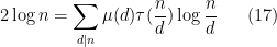
So we see that when trying to sum the von Mangoldt function by elementary means, the error term overwhelms the main term . But there is a slight tweaking of the von Mangoldt function, the second von Mangoldt function  , that increases the size of the main term to
  while keeping the error term at , thus leading to a useful estimate; the price one pays for this is that this function is now a proxy for the almost primes rather than the primes. This function is defined by a variant of (10), namely

It is not hard to see that  vanishes once has at least three distinct prime factors (basically because the quadratic function
  vanishes after being differentiated three or more times). Indeed, one can easily verify the identity

(which corresponds to the Dirichlet series identity  ); the first term
  is mostly concentrated on primes, while the second term
  is mostly concentrated on semiprimes (products of two distinct primes).
Now let us sum . In analogy with the previous discussion, we will do so by comparing the function  with something involving the divisor function. In view of (5), it is reasonable to try the approximation
from the identity
(which corresponds to the Dirichlet series identity  ) we thus expect
Now we make these heuristics more precise. From the integral test we have

while from (9) and summation by parts one has

where  are explicit absolute constants whose exact value is not important here. Thus

for some other constants  .
.
Meanwhile, from (15), (17) one has

applying (19), (13), (14) we see that the right-hand side is . Computing  by the integral test, we deduce the Selberg symmetry formula

One can view (20) as the “almost prime number theorem” – the analogue of the prime number theorem for almost primes.
The fact that the almost primes have a relatively easy asymptotic, while the genuine primes do not, is a reflection of the parity problem in sieve theory; see this post for further discussion. The symmetry formula is however enough to get “within a factor of two” of the prime number theorem: if we discard the semiprimes  from (16), we see that
  , and thus

which by a summation by parts argument leads to

which is within a factor of of (2) in some sense.
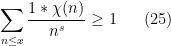
One can “twist” all of the above arguments by a Dirichlet character . For instance, (15) twists to

On the other hand, if is a non-principal character of modulus , then it has mean zero on any interval with length , and it is then not hard to establish the asymptotic

This soon leads to the twisted version of (20):

thus almost primes are asymptotically unbiased with respect to non-principal characters.
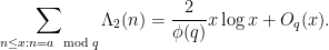
From the multiplicative Fourier analysis of Dirichlet characters modulo (and the observation that is quite small on residue classes not coprime to ) one then has an “almost prime number theorem in arithmetic progressions”:
As before, this lets us come within a factor of two of the actual prime number theorem in arithmetic progressions:

One can also twist things by the completely multiplicative function  , but with the caveat that the approximation
  to can locally correlate with . Thus for instance one has
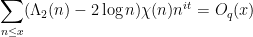
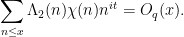
for any fixed and ; in particular, if is non-principal, one has
— 3. The all-or-nothing dichotomy —
To summarise so far, the almost primes (as represented by ) are quite uniformly distributed. These almost primes can be split up into the primes (as represented by ) and the semiprimes (as represented by ), thanks to (16).
One can rewrite (16) as a recursive formula for :

One can also twist this formula by a character and/or a completely multiplicative function , thus for instance

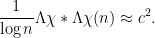
This recursion, combined with the uniform distribution properties on , lead to various all-or-nothing dichotomies for . Suppose, for instance, that  behaves like a constant
  on the average for some non-principal character :

Then (from (5)) we expect  to behave like
  , thus
On the other hand, from (21),  is asymptotically uncorrelated with :

Putting all this together, one obtains

which suggests that must be either close to , or close to .
Basically, the point is that there are only two equilibria for the recursion (23). One equilibrium occurs when is asymptotically uncorrelated with ; the other is when it is completely anti-correlated with , so that is supported primarily on those for which is close to . Note in the latter case  for most primes , and thus
  for most semiprimes , thus leading to an equidistribution of for almost primes (weighted by ). Any intermediate distribution of would be inconsistent with the distribution of
  . (In terms of Dirichlet series, this assertion corresponds to the fact that the -function of either has a zero of order , or a zero of order (i.e. not a zero at all) at .)
A similar phenomenon occurs when twisting by ; basically, the average value of  must asymptotically either be close to , or close to ; no other asymptotic ends up being compatible with the distribution of
  . (Again, this corresponds to the fact that the Riemann zeta function has a zero of order or at .) More generally, the average value of
 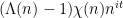 must asymptotically approach either or .
Remark 2 One can make the above heuristics precise either by using Dirichlet series (and analytic continuation, and the theory of zeroes of meromorphic functions), or by smoothing out arithmetic functions such as by a suitable multiplicative convolution with a mollifier (as is basically done in elementary proofs of the prime number theorem); see also the Granville-Soundararajan theory of pretentious characters for a closely related theory. We will not pursue these details here, however.
— 4. Dueling conspiracies —
In the previous section we have seen (heuristically, at least), that the von Mangoldt function (or more precisely,  ) will either have no correlation, or a maximal amount of anti-correlation, with a completely multiplicative function such as , , or
  . On the other hand, it is not possible for this function to maximally anti-correlate (or to conspire) with two such functions; thus the presence of one conspiracy excludes the presence of all others.
Suppose for instance that we had two distinct non-principal characters  for which one had maximal anti-correlation:

One could then combine the two statements to obtain

Meanwhile, doesn’t correlate with either or  . It will be convenient to exploit this to normalise , obtaining

(Note from (3), (18) that we expect  to have mean zero.)
On the other hand, since  , one has
and hence by the triangle inequality

in the sense that averages of the left-hand side should be at least as large as averages of the right-hand side. From this, (18), and Cauchy-Schwarz, one thus expects

But if one expands out the left-hand side using (18), (21), one only ends up with  on the average, a contradiction for sufficiently large.
Remark 3 The above argument belongs to a family of  -based arguments which go by various names (almost orthogonality,
  , large sieve, etc.). The argument can more generally be used to establish square-summability estimates on averages such as
  as varies, but we will not make this precise here.
As one consequence of the above arguments, one can show that cannot maximally anti-correlate with any non-real character , since (by the reality of ) it would then also maximally anti-correlate with the complex conjugate  , which is distinct from . A similar argument shows that cannot maximally anti-correlate with for any non-zero , a fact which can soon lead to the prime number theorem, either by Dirichlet series methods, by Fourier-analytic means, or by elementary means. (Sketch of Fourier-analytic proof: methods provide -type bounds on the averages of
  in , while the above arguments show that these averages are also small in
  . Applying (22) a few times to take advantage of the smoothing effects of convolution, one eventually concludes that these averages can be made arbitrarily small in
  asymptotically, at which point the prime number theorem follows from Fourier inversion.)
Remark 4 There is a slightly different argument of an nature rather than an nature (i.e. using tools such as the triangle inequality, union bound, etc.) that can also achieve similar results. For instance, suppose that maximally anti-correlates with and . Then  for most primes , which implies that
  for most primes , which is incompatible with the all-or-nothing dichotomy unless
  is principal. This is an alternate way to exclude correlation with non-real characters. Similarly, if
  , then
  , which is also incompatible with the zero-one law; this is essentially the method underlying the standard proof of the prime number theorem (which relates
  with
with  ).
).
— 5. Quadratic characters —
The one difficult scenario to eliminate is that of maximal anti-correlation with a real non-principal (i.e. quadratic) character , thus
This scenario implies that the quantity

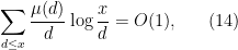
vanishes. Indeed, if one starts with the identity
and sums in , one sees that

The left-hand side is  by the mean zero and periodicity properties of . To estimate the right-hand side, we use the hyperbola method and rewrite it as

for some parameter  (sufficiently slowly growing in ) to be optimised later. Writing
  and
and  , we can express this as

sending (and  at a slower rate) we conclude
  as required.
It is remarkably difficult to show that  does not, in fact, vanish. One way to do this is to use the class number formula, that relates this quantity to the class number of the quadratic number field
  associated to the conductor of , together with some related number-theoretic quantities. A more elementary (but significantly weaker) method proceeds by using the easily verified fact that the convolution
  is non-negative, and is at least on the squares; this should be interpreted as a fact from algebraic number theory, and basically corresponds to the fact that the number of representations of an integer as the norm
  of an integer in
  (or more generally, as the norm of an ideal in that ring) is non-negative, and is at least on the squares. In particular we have
On the other hand, from the hyperbola method we can express the left-hand side as

From the mean zero and periodicity properties of we have  , so the second term in (24) is
  . Meanwhile, from the midpoint rule,
  , and so the first term in (24) is
Putting all this together we have

which leads to a contradiction as if vanishes.
Note in fact that the above argument shows that is positive. If one carefully computes the dependence of the above argument on the modulus , one obtains a lower bound of the form  , which is quite poor. Using a non-trivial improvement on the error term in counting lattice points under the hyperbola (or better still, by smoothing the sum
  ), one can improve this a bit, to
  . In contrast, the class number method gives a bound
  .
.
We can improve this even further for all but at most one real primitive character :
Theorem 1 (Siegel’s theorem) For every  , one has
  for all but at most one real primitive character , where the implied constant is effective, and is the modulus of .
Throwing in this (hypothetical) one exceptional character, we conclude that for all real primitive characters , but now the implied constant is ineffective, which is the usual way in which Siegel’s theorem is formulated (but the above nearly effective refinement can be obtained by the same methods). It is a major open problem in the subject to eliminate this exceptional character and recover an effective estimate for some  .
.
Proof: Let (which we can assume to be small), and let  be a small number depending (effectively) on
  to be chosen later. Our task is to show that
  for all but at most one primitive real character . Note we may assume is large (effectively) depending on , as the claim follows from the previous bounds on otherwise.
Suppose then for contradiction that  and
and  for two distinct primitive real characters of (large) modulus
  respectively.
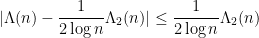
We begin by modifying the proof that was positive, which relied (among other things) on the observation that  , and equals at . In particular, one has
for any  and any real . (One can get slightly better bounds by exploiting that is also at least on square numbers, as before, but this is really only useful for
  , and we are now going to take much closer to .)
On the other hand, one has the asymptotics
for any real close (but not equal) to , and similarly
for any real close to ; similarly for  . From the hyperbola method, we can then conclude

for all real sufficiently close to . Indeed, one can expand the left-hand side of (26) as

and the claim then follows from the previous asymptotics. (One can improve the error term by smoothing the summation, but we will not need to do so here.)
Now set  for a large absolute constant
  . If
. If  , then the error term in
  is then at most
  (say) if is large enough. We conclude from (25) that

for . Since  and is assumed small (depending on ), this implies that
  is positive in the range

(this can be seen by checking the cases  and
and  separately). On the other hand, has a simple pole at with positive residue, and is thus negative for
  extremely close to . By the intermediate value theorem, we conclude that
  has a zero for some
  . Conversely, it is not difficult (using summation by parts) to show that
  for
for  , and so by the mean value theorem we see that the zero of must also obey
  . Thus has a zero for some
  with
with

Similarly,  has a zero for some
  with
with

Now, we consider the function

One can also show that  is non-negative and equals at , thus

(The algebraic number theory interpretation of this positivity is that is the number of representations of as the norm of an ideal in the biquadratic field generated by  and
and  .)
.)
Also, by (a more complicated version of) the derivation of (26), one has

(say). Arguing as before, we conclude that

for . Using the bound  (which can be established by summation by parts), we conclude that
  is positive in the range

Since we already know and have zeroes for some  obeying (27), (28)

taking geometric means and rearranging we obtain

But this contradicts the hypotheses ,  if is small enough.
Remark 5 Siegel’s theorem leads to a version of the prime number theorem in arithmetic progressions known as the Siegel-Walfisz theorem. As with Siegel’s theorem, the bounds are ineffective unless one is allowed to exclude a single exceptional modulus (and its multiples), in which case one has a modified prime number theorem which favours the quadratic nonresidues mod ; see this paper of Granville.
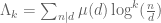
Remark 6 One can improve the effective bounds in Siegel’s theorem if one is allowed to exclude a larger set of bad moduli. For instance, the arguments in Section 4 allow one to establish a bound of the form  after excluding at most one in each hyper-dyadic range
  for each ; one can of course replace
  by other exponents here, but at the cost of worsening the term. (This is essentially an observation of Landau.)


35 comments
Comments feed for this article
24 September, 2009 at 7:05 pm
David Speyer
Very nice exposition!
(1) I remember reading that, before the classification of imaginary quadratic fields of class number 1 was proved, it was known that there could be at most one example in addition to the ones already known. Is that the same “at most one”?
(2) If you felt like expanding Remark 1 into a blog post, I would certainly be interested in reading it.
25 September, 2009 at 1:49 am
Terence Tao
(1) Yes, this is very closely related, though I think the discovery that there is at most one exceptional field of class number 1 predates Siegel’s theorem slightly. The elimination of this field is quite difficult (it can’t be done by the methods discussed here), but I don’t know many details.
(2) Actually I was already thinking of doing something along those lines, though perhaps not immediately…
26 September, 2009 at 6:06 pm
anon
Thanks for an excellent posting.
A minor expository point: the numbers 0 and 1 occur in the initial discussion of the “zero-one law”, in a way which (to any reader not already knowing the term) reinforces but also confuses the meaning of the term here. In the original probability context, 0 and 1 had meaning as probabilities, but in the present situation it just refers to an all-or-nothing dichotomy of possible asymptotic behaviors.
26 September, 2009 at 6:33 pm
Terence Tao
Hmm, that’s a fair point. It’s a shame that the term “zero-one law” is so narrowly defined, because I find it a useful phrase in other contexts. I wonder if anyone can suggest a replacement term; “all-or-nothing dichotomy” is OK, I guess, but perhaps a little clunky.
30 September, 2009 at 6:04 pm
Terence Tao
I’ve gone ahead and replaced “zero-one law” with “all-or-nothing dichotomy”; this is not my ideal terminology, but will serve as a placeholder until a better suggestion comes along.
I also fixed an error in which the rings![Z[\sqrt{q}]](https://s0.wp.com/latex.php?latex=Z%5B%5Csqrt%7Bq%7D%5D&bg=ffffff&fg=545454&s=0&c=20201002) and
and ![Z[\sqrt{-q}]](https://s0.wp.com/latex.php?latex=Z%5B%5Csqrt%7B-q%7D%5D&bg=ffffff&fg=545454&s=0&c=20201002) were confused. (At some point in the future I plan to learn class field theory properly, and perhaps blog about it here; my algebraic number theory knowledge is unfortunately still rather superficial at present.)
were confused. (At some point in the future I plan to learn class field theory properly, and perhaps blog about it here; my algebraic number theory knowledge is unfortunately still rather superficial at present.)
1 October, 2009 at 6:52 pm
same anon
(from the anon who posted the earlier 0-1 comment)
Actually, “zero-one law” is too good a metaphor to not use. It works beautifully for any reader who already understands the meaning. Not only does it convey the idea, but seeing the term used here outside its traditional settings also suggests the idea of spreading that usage to other contexts.
The only caveat is that readers who aren’t already familiar with the idea would probably benefit if, at the first location in the essay where “0-1 law” appears, there were also:
— an aside, giving a definition or a few words of explanation (e.g., “borrowing a metaphor from the 0-1 laws of probability”);
— disambiguation, in the discussion that follows of the order of vanishing of the associated Dirichlet series being either 0 or 1 and this being an avatar of the 0-1 law, that these orders being “0” and “1” (in whichever order corresponds to the dichotomy in the 0-1 law!) is just a numerical peculiarity of this problem and is otherwise unrelated to the words in the term “zero-one law”.
I guess it also bears clarifying what a 0-1 law is, in general. I don’t think the meaning is simply that of a dichotomy, there is also some dynamics driving the outcome, asymptotically, to one of two antipodal equilibria (indeed you call the two values of $c$ “equilibria”, so maybe you share the same intuition). This is literally or tacitly true in every theorem I can remember being called a 0-1 law (in probability, random graphs, ergodic theory, information theory, etc), and it would be interesting to make a list and see whether this dynamical, asymptotic aspect is always part of the story.
26 September, 2009 at 11:05 pm
Anonymous
Near the beginning, when you say that the number of primes congruent to a mod q when a is not coprime to q is O(1), you can leave out the dependence of the implied constant on q. [Well spotted, thanks! -T.]
27 September, 2009 at 4:37 pm
Mustafa Said
One open problem in analytic number theory is to determine whether or not $\sum_1^{\infty} (-1)^n \frac{n}{p_n}$ converges. Here $p_n$ denotes the $n^th$ prime. The prime number theorem gives us some information on the asymptotics of the terms in the sum, but not enough to solve the problem. Would the validity of the Riemann Hypothesis help us solve this problem?
30 September, 2009 at 4:10 pm
Terence Tao
Hmm. I played around with this sum a bit and it seems like the convergence of this sum is equivalent to the convergence of the sum (by using the prime number theorem and estimating the difference between
  and
and  for odd and even n.) So it comes down to understanding the equidistribution of the parity of the prime counting function; roughly speaking, any quantatitative equidistribution which gains more than a log log factor should suffice. By coincidence, we happen to be studying the parity of pi(x) over at the polymath4 project, though I don’t think the methods we have currently for computing that parity are strong enough to establish this sort of equidistribution. Nevertheless it does seem plausible (though difficult to prove) that one has convergence. (If one had a sufficiently uniform and quantitative version of the Poisson statistics conjecture for prime gaps, one might be able to obtain the result; in particular, a sufficiently quantitative version of the prime tuples conjecture might suffice, thanks to Gallagher’s computations relating the two.)
The Riemann hypothesis concerns larger-scale fluctuations in the primes, whereas here it seems that fine-scale fluctuations such as prime gaps statistics are more relevant.
7 March, 2010 at 6:14 pm
Mustafa Said
Can you please explain your statement “any quantatitative equidistribution (of the parity of the prime counting function) which gains more than a log log factor should suffice.”
I also have another question about the parity of the prime counting
function:
Let $E_N = { m \in \mathbb{N} : \pi(m) is even and m \leq N}$
and $O_N = { m \in \mathbb{N} : \pi(m) is odd and m \leq N}
then is it true that $\lim_{N \to \infty} |E_N|/|O_N| = 1$ ?
28 September, 2009 at 9:19 am
Anonymous
There are lots of ways you can use the phrase “all or nothing.” You can say all-or-nothing behavior, all-or-nothing phenomenon, all-or-nothing situation, etc. Another expression you can use in place of all or nothing is “black or white” — as in no shades of gray. One reason “all-or-nothing dichotomy” seems clunky is that it is redundant.
1 October, 2009 at 8:11 pm
Arithmetic Progression in finite fields
Professor Tao:
I have a particular problem that is of interest in electrical engineering. It seems to fall under the category of arithmetic progression but in finite fields.
Field field: F_{p^n} with n>1
What is the maximum N so that one can find N different polynomials
p_{i}(x) of degree in F_{p}[x] for i = 1,…,N so that the following
conditions are satisfied?
1) each p_{i}(x) has at least 2^n roots in F_{p^n} in arithmetic
progression. By AP what I mean is: let s be primitive element. If r is
root, then r, r+1, r+s, r+1+s,r+s^2, r+s^2+1, r+s^2+s,
r+s^2+s+1,…,r+s^(n-1)+s^(n-2)+…+1 are roots.
2) If i is not j, p_{i}(x) and p_{j}(x) should have no common roots
from the roots in arithmetic progression.
As n increases from 0 to infinity what is the highest such N one can
get for each F_{p^n}?
(I could not get more than N=5 for p=5. For p=3, N=1.)
Is there any mathematician who has worked on problems involving such progressions in finite fields?
Thank you
2 October, 2009 at 3:42 pm
At the AustMS conference « What’s new
[…] follows from (for instance) Siegel’s theorem on the size of the class group, as discussed in this previous post. Ellenberg, Venkatesh, and Westerland have recently established some partial results towards the […]
6 October, 2009 at 4:36 pm
Giampiero Campa
Hi Terry,
first of all i am an not a Mathematician, so i’d like to apologize in advance if the language i am using is not entirely correct or appropriate.
Let me put it this way, do we “understand”, say, the Mandelbrot fractal ? I mean, yes we do have a dynamic system that generates it, but as far as i know the only way we can determine whether a point belongs to the set or not is by iterating the dynamic system. Isn’t that somehow similar to the situation that we have with prime numbers where the only way to find out if a number is prime or not is by going through the sieve ? or simply dividing the number by all its predecessors ? (which i am pretty sure it can be done with a simple 1-state nonlinear dynamic system)
In other words, are we expecting too much by saying, as you did in your first sentence, that we want to “understand the distribution of prime numbers” ?
Again, maybe these are trivial questions and i just don’t know enough number theory, in which case i apologize.
28 June, 2012 at 7:23 am
K
Somewhat like, to see if a living creature is a human being, it’s a good idea to test its DNA, but perhaps it’s not very useful for the understanding of the distribution of people in the world…
6 November, 2009 at 7:49 am
The “no self-defeating object” argument « What’s new
[…] 1 Continuing the number-theoretic theme, the “dueling conspiracies” arguments in a previous blog post can also be viewed as an instance of this type of “no-self-defeating-object”; for […]
23 July, 2011 at 7:40 pm
Erdos’ divisor bound « What’s new
[…] requires one to exclude zeroes of the Riemann zeta function on the line , as discussed in this previous post), one is eventually left with the estimate , which is useless as a lower bound (and recovers only […]
21 August, 2011 at 12:45 pm
Hilbert’s seventh problem, and powers of 2 and 3 « What’s new
[…] (The reason the Thue-Siegel-Roth theorem is ineffective is because it relies heavily on the dueling conspiracies argument, i.e. playing off multiple “conspiracies” against each other; the other results […]
11 November, 2011 at 1:18 pm
Number Theory: Lecture 16 « Theorem of the week
[…] there was no known elementary proof when the first edition was written!). Terry Tao has a nice blog post discussing a number of aspects of the distribution of prime […]
19 April, 2012 at 7:23 pm
Sumit Kumar Jha
Professor Tao:


Your derivation of Selberg’s symmetry formula is the one which Selberg originally used in his derivation of an elementary proof of prime number theorem.
But in a paper by Iseki and Tatsukava, they easily derived
and this is equivalent to
where
Can you help me to deduce
from above equation.
19 April, 2012 at 7:38 pm
Sumit Kumar Jha
Actually,
 when
when 
 when
when 
 when
when 
 in other cases.
but how is it that
20 April, 2012 at 5:15 am
Terence Tao
This follows from the formula in your previous comment.
20 April, 2012 at 7:22 am
Sumit Kumar Jha
Professor Tao: Thanks!!
 .
.
I am also looking forward for an article on “sieves” on your blog. Have you already written one??
I especially want to know about the Bomberi sieve which treats
Can you also discuss the departure from “almost primes” to “primes” namely parity problem in detail??
20 May, 2012 at 2:58 pm
Heuristic limitations of the circle method « What’s new
[…] the only thing which is strong enough to rule out a conspiracy is a conflicting conspiracy (see my previous blog post on this topic). A good example of this is Heath-Brown’s result that the existence of a Siegel zero (which […]
27 June, 2012 at 8:25 am
What if primes hated to start with nine? « Secret Blogging Seminar
[…] appeared earlier in an answer I left on MO. There is also a lot of similarity to Terry Tao’s post on conspiracies and the prime number theorem. One can think of “primes hate to start with nine” as a “conspiracy” whose […]
27 November, 2012 at 9:04 pm
Sujit Nair
Typo: There should be a instead of
  in the rightmost term in the equation above (8)
[Corrected, thanks – T.]
19 July, 2013 at 2:31 pm
The Riemann hypothesis in various settings | What's new
[…] e.g. this previous blog post for more […]
15 November, 2013 at 3:15 am
Number Theory: Lecture 16 | Theorem of the week
[…] there was no known elementary proof when the first edition was written!). Terry Tao has a nice blog post discussing a number of aspects of the distribution of prime […]
11 December, 2013 at 11:50 am
Mertens’ theorems | What's new
[…] on the Riemann zeta function in the neighbourhood of the pole at , whereas (as discussed in this previous post) the prime number theorem requires control on the zeta function on (a neighbourhood of) the line . […]
7 July, 2014 at 2:20 am
The subspace theorem approach to Siegel’s theorem on integral points on curves via nonstandard analysis | What's new
[…] an effective bound may be easily established). This is ultimately due to the reliance on the “dueling conspiracy” (or “repulsion phenomenon”) strategy. We do not as yet have a good way to rule […]
24 September, 2014 at 2:29 pm
Derived multiplicative functions | What's new
[…] a key role in the Erdös-Selberg elementary proof of the prime number theorem (as discussed in this previous blog post), is the top order term of the […]
9 December, 2014 at 6:05 pm
Anonymous
Prof Tao
I was wondering how exactly the summation by parts works to get equation (2) from prime number theorem ? Thanks.
[This is an instructive exercise and I recommend that you try your hand at it. You can take a look at the proof of Theorem 36 of https://terrytao.wordpress.com/2014/11/23/254a-notes-1-elementary-multiplicative-number-theory/ for some related arguments. -T.]
17 June, 2015 at 7:50 am
The prime tuples conjecture, sieve theory, and the work of Goldston-Pintz-Yildirim, Motohashi-Pintz, and Zhang | fragments
[…] annoyingly, the implied constant here is only ineffectively bounded with current methods; see this previous post for further […]
12 November, 2015 at 8:20 am
Klaus Roth | What's new
[…] when the denominators are very different in size. (I refer to this sort of argument as a “dueling conspiracies” argument; they are strangely prevalent throughout analytic number […]
5 December, 2021 at 1:48 pm
Sam Li
Great post. Minor thing: The link to PlanetMath for “Dirichlet hyperbola method” has inevitably rotted.
[Corrected, thanks -T.]