
Analytic number theory is often concerned with the asymptotic behaviour of various arithmetic functions: functions 


Regardless of what commutative ring
An important class of arithmetic functions in analytic number theory are the multiplicative functions, that is to say the arithmetic functions 
for all coprime 


- the Kronecker delta
, defined by setting
for
and
otherwise;
- the constant function
and the linear function
(which by abuse of notation we denote by
);
- more generally monomials
for any fixed complex number
(in particular, the “Archimedean characters”
for any fixed
), which by abuse of notation we denote by
;
- Dirichlet characters
;
- the Liouville function
;
- the indicator function of the
–smooth numbers (numbers whose prime factors are all at most
- the indicator function of the
Examples of multiplicative functions that are not completely multiplicative include
- the Möbius function
;
- the divisor function
(also referred to as
);
- more generally, the higher order divisor functions
for
;
- the Euler totient function
;
- the number of roots
of a given polynomial
defined over
;
- more generally, the point counting function
of a given algebraic variety
defined over
- the function
that counts the number of representations of
- more generally, the function that maps a natural number
of absolute norm
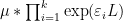
These multiplicative functions interact well with the multiplication and convolution operations: if 


Finally, the product of completely multiplicative functions is again completely multiplicative. On the other hand, the sum of two multiplicative functions will never be multiplicative (just look at what happens at
The specific multiplicative functions listed above are also related to each other by various important identities, for instance

where 
On the other hand, analytic number theory also is very interested in certain arithmetic functions that are not exactly multiplicative (and certainly not completely multiplicative). One particularly important such function is the von Mangoldt function 


Definition 1 A derived multiplicative function
at the origin of a family
of multiplicative functions
parameterised by a formal parameter
. Equivalently,
of
such that the arithmetic function
is multiplicative, or equivalently that
is multiplicative and one has the Leibniz rule
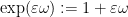
More generally, for any
, a
-derived multiplicative function
at the origin of a family
of multiplicative functions
parameterised by formal parameters
. Equivalently,
coefficient of a multiplicative function in the extension
of
We define the notion of a


There are Leibniz rules similar to (2) but they are harder to state; for instance, a doubly derived multiplicative function 


for all coprime
One can then check that the von Mangoldt function 
![{{\bf C}[\varepsilon]/(\varepsilon^2)}](https://s0.wp.com/latex.php?latex=%7B%7B%5Cbf+C%7D%5B%5Cvarepsilon%5D%2F%28%5Cvarepsilon%5E2%29%7D&bg=ffffff&fg=000000&s=0&c=20201002)


Remark 1 One can also phrase these concepts in terms of the formal Dirichlet series
associated to an arithmetic function
Using the definition of a 


![{C[\varepsilon_1,\dots,\varepsilon_k]/(\varepsilon_1^2,\dots,\varepsilon_k^2)}](https://s0.wp.com/latex.php?latex=%7BC%5B%5Cvarepsilon_1%2C%5Cdots%2C%5Cvarepsilon_k%5D%2F%28%5Cvarepsilon_1%5E2%2C%5Cdots%2C%5Cvarepsilon_k%5E2%29%7D&bg=ffffff&fg=000000&s=0&c=20201002)
It then turns out that most (if not all) of the basic identities used by analytic number theorists concerning derived multiplicative functions, can in fact be viewed as coefficients of identities involving purely multiplicative functions, with the latter identities being provable primarily from multiplicative identities, such as (1). This phenomenon is analogous to the one in linear algebra discussed in this previous blog post, in which many of the trace identities used there are derivatives of determinant identities. For instance, the Leibniz rule

for any arithmetic functions 

in the ring with one infinitesimal 

are top order terms of

and the variant formula 

which can then be deduced from the previous identities by noting that the completely multiplicative function 


which plays a key role in the Erdös-Selberg elementary proof of the prime number theorem (as discussed in this previous blog post), is the top order term of the identity

involving the multiplicative functions 


and (1). Similarly for higher identities such as

which arise from expanding out 
An analogous phenomenon arises for identities that are not purely multiplicative in nature due to the presence of truncations, such as the Vaughan identity

for any 


which can be easily derived from the identities 


valid for natural numbers up to 


and arises by first observing that

vanishes up to 
One consequence of this phenomenon is that identities involving derived multiplicative functions tend to have a dimensional consistency property: all terms in the identity have the same order of derivation in them. For instance, all the terms in the Selberg symmetry formula (3) are doubly derived functions, all the terms in the Vaughan identity (4) or the Heath-Brown identity (5) are singly derived functions, and so forth. One can then use dimensional analysis to help ensure that one has written down a key identity involving such functions correctly, much as is done in physics.
In addition to the dimensional analysis arising from the order of derivation, there is another dimensional analysis coming from the value of multiplicative functions at primes 


A 
By taking top order coefficients, we then see that the convolution of a 


One caveat, though: this latter dimensional consistency breaks down for identities that involve infinitely many terms, such as Linnik’s identity
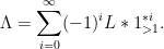
In this case, one can still rewrite things in terms of multiplicative functions as

so the former dimensional consistency is still maintained.
I thank Andrew Granville, Kannan Soundararajan, and Emmanuel Kowalski for helpful conversations on these topics.

20 comments
Comments feed for this article
24 September, 2014 at 2:59 pm
Eytan Paldi
It seems that the sum of two multiplicative functions can be multiplicative only if one of them is the constant function .
.
[By definition, multiplicative functions are required to take the value at
at  . -T.]
24 September, 2014 at 3:30 pm
Anonymous
Dear Prof. Tao, My browser (IE) mentions a parsing error for the formula preceding Remark 1.
[Corrected, thanks – T.]
24 September, 2014 at 6:59 pm
ACB
Should the second j in the sentence beginning, “Note that the convolution of a multiplicative function…” be a j’?
[Corrected, thanks – T.]
25 September, 2014 at 5:44 am
MrCactu5 (@MonsieurCactus)
If you don’t like the language of nilpotents, maybe just use matrices? Your epsilon can be written as
0 1
0 0
27 September, 2014 at 5:55 pm
David Roberts
Wouldn’t Hecke operators on modular curves be an example of a multiplicative function
  , considered as a map to endomorphisms of modular forms?
28 September, 2014 at 7:47 am
Terence Tao
Yes, this is an example. It looks like the corresponding endomorphism-valued Dirichlet series generates scalar Dirichlet series associated to various modular forms as coefficients using a basis of Hecke eigenforms, though this statement is basically tautological and I don’t know if one can do much with it that one can’t already do with the usual formulation of Hecke operators and eigenforms.
9 October, 2014 at 7:34 am
valuevar
Very nice! I was just wondering the other day – is there a name for the “higher identities” such as the one involving ? (I know about Diamond-Steinig identities for
  .) I thought these identities were somehow associated with Bombieri, but that may be an association that existed partly in my head. (I’ve also heard some people crediting them to Faa di Bruno, who wrote down a chain rule for higher derivatives in the nineteenth century, but was not the first to do so.)
9 October, 2014 at 8:00 am
Terence Tao
The identity explicitly appears in this 1975 paper of Bombieri: http://matwbn.icm.edu.pl/ksiazki/aa/aa28/aa2828.pdf . I don’t know if this is the earliest explicit appearance of it, though. For instance, Selberg already (implicitly) used the k=2 version of this formula in his 1949 proof of the prime number theorem in http://www.jstor.org/stable/1969455 , so I would find it plausible that he was aware of some version of the higher k identity also (but perhaps using different notation than the now-standard
  ). Actually, I think the use of
  as a tool to detect k-almost primes even predates Selberg, though I’ll have to track down a precise reference for this…
[UPDATE: I found the reference, but it turns out to postdate Selberg by a little bit: a close relative of the above identity appears in the 1956 PhD thesis of Golomb, “Problems in the distribution of the prime numbers”, in which it is observed that whenever
  are coprime; see http://www.sciencedirect.com/science/article/pii/0022314X70900193 .]
13 October, 2014 at 12:40 am
valuevar
This is helpful; thanks. However, for several applications (including at least some of those of Selberg, I believe) an identity involving $L^k\mu \ast 1$ has got $L^k$ attached to the wrong factor; it is much nicer to have it attached to $1$ rather than to $\mu$.
13 October, 2014 at 4:31 am
Mats Granvik
Möbius function calculated from arbitrary numbers as input:
http://math.stackexchange.com/questions/268159/m%c3%b6bius-function-from-random-number-sequence
27 November, 2014 at 7:58 pm
Fan
The use of and
and  is inconsistent in Definition 1.
[Corrected, thanks – T.]
11 January, 2015 at 12:19 pm
Top 30 Computer Science and Programming Blogs | Yo Worlds
[…] 14. Terry Tao’s Blog: Terry Tao is a mathematician whose work is frequently relevant for computer scientists and computational theorists. Most of the posts are highly technical mathematical demonstrations that are not accessible to layman. This makes his blog an intellectually challenging but fruitful endeavor for the serious student of computer science or mathematics. Highlight: Derived Multiplicative Functions […]
17 May, 2015 at 7:11 am
Топ-30 лучших блогов о программировании… | IT News
[…] Что почитать на Terry Tao’s Blog: Производные мультипликативные функции […]
17 October, 2015 at 1:12 am
BLOGS ON COMPUTER SCIENCE | CS SECTION 6B 2013
[…] 14. Terry Tao’s Blog: Terry Tao is a mathematician whose work is frequently relevant for computer scientists and computational theorists. Most of the posts are highly technical mathematical demonstrations that are not accessible to layman. This makes his blog an intellectually challenging but fruitful endeavor for the serious student of computer science or mathematics. Highlight: Derived Multiplicative Functions […]
30 August, 2016 at 4:10 pm
Heuristic computation of correlations of the divisor function | What's new
[…] We remark that is an example of a derived multiplicative function, discussed in this previous blog post. […]
22 September, 2016 at 8:45 am
254A, Notes 1: Elementary multiplicative number theory | What's new
[…] also considers arithmetic functions taking values in more general rings than or , as in this previous blog post, but we will restrict attention here to the classical situation of real ofr complex arithmetic […]
31 October, 2017 at 9:08 pm
Computer science – Live Free
[…] 14. Terry Tao’s Blog: Terry Tao is a mathematician whose work is frequently relevant for computer scientists and computational theorists. Most of the posts are highly technical mathematical demonstrations that are not accessible to layman. This makes his blog an intellectually challenging but fruitful endeavor for the serious student of computer science or mathematics. Highlight: Derived Multiplicative Functions […]
27 November, 2017 at 3:55 am
Топ-30 лучших блогов о программировании и вычислительной технике — Rus.Rocks
[…] Что почитать на Terry Tao’s Blog: Производные мультипликативные функции […]
13 December, 2017 at 9:27 am
Sean Lynch
Regarding remark 1, do you mean the logarithmic derivative of an Euler product?
[Corrected, thanks – T.]
19 January, 2021 at 4:46 am
asahay22
Unless I’ve misunderstood something, it appears to me that 1-derived multiplicative functions are precisely the functions that arise as the coefficients of in for a multiplicative function
 ![f:\mathbb{N} \to \mathbb{C}[[x]]](https://s0.wp.com/latex.php?latex=f%3A%5Cmathbb%7BN%7D+%5Cto+%5Cmathbb%7BC%7D%5B%5Bx%5D%5D&bg=ffffff&fg=545454&s=0&c=20201002) . This raises the question that do functions that are the coefficients of
. This raises the question that do functions that are the coefficients of  for
for  as above arise in analytic number theory or sieve theory?
Also, a minor point, but I think you intended to use in the paragraph right after Remark 1.