254A, Notes 3: The large sieve and the Bombieri-Vinogradov theorem

A fundamental and recurring problem in analytic number theory is to demonstrate the presence of cancellation in an oscillating sum, a typical example of which might be a correlation

between two arithmetic functions and , which to avoid technicalities we will assume to be finitely supported (or that the variable is localised to a finite range, such as ). A key example to keep in mind for the purposes of this set of notes is the twisted von Mangoldt summatory function

that measures the correlation between the primes and a Dirichlet character . One can get a “trivial” bound on such sums from the triangle inequality

for instance, from the triangle inequality and the prime number theorem we have

as . But the triangle inequality is insensitive to the phase oscillations of the summands, and often we expect (e.g. from the probabilistic heuristics from Supplement 4) to be able to improve upon the trivial triangle inequality bound by a substantial amount; in the best case scenario, one typically expects a “square root cancellation” that gains a factor that is roughly the square root of the number of summands. (For instance, for Dirichlet characters of conductor , it is expected from probabilistic heuristics that the left-hand side of (3) should in fact be for any .)

It has proven surprisingly difficult, however, to establish significant cancellation in many of the sums of interest in analytic number theory, particularly if the sums do not have a strong amount of algebraic structure (e.g. multiplicative structure) which allow for the deployment of specialised techniques (such as multiplicative number theory techniques). In fact, we are forced to rely (to an embarrassingly large extent) on (many variations of) a single basic tool to capture at least some cancellation, namely the Cauchy-Schwarz inequality. In fact, in many cases the classical case

considered by Cauchy, where at least one of is finitely supported, suffices for applications. Roughly speaking, the Cauchy-Schwarz inequality replaces the task of estimating a cross-correlation between two different functions , to that of measuring self-correlations between and itself, or and itself, which are usually easier to compute (albeit at the cost of capturing less cancellation). Note that the Cauchy-Schwarz inequality requires almost no hypotheses on the functions or , making it a very widely applicable tool.

There is however some skill required to decide exactly how to deploy the Cauchy-Schwarz inequality (and in particular, how to select and ); if applied blindly, one loses all cancellation and can even end up with a worse estimate than the trivial bound. For instance, if one tries to bound (2) directly by applying Cauchy-Schwarz with the functions and , one obtains the bound

The right-hand side may be bounded by , but this is worse than the trivial bound (3) by a logarithmic factor. This can be “blamed” on the fact that and are concentrated on rather different sets ( is concentrated on primes, while is more or less uniformly distributed amongst the natural numbers); but even if one corrects for this (e.g. by weighting Cauchy-Schwarz with some suitable “sieve weight” that is more concentrated on primes), one still does not do any better than (3). Indeed, the Cauchy-Schwarz inequality suffers from the same key weakness as the triangle inequality: it is insensitive to the phase oscillation of the factors .

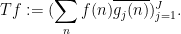
While the Cauchy-Schwarz inequality can be poor at estimating a single correlation such as (1), its power improves when considering an average (or sum, or square sum) of multiple correlations. In this set of notes, we will focus on one such situation of this type, namely that of trying to estimate a square sum

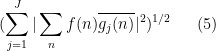
that measures the correlations of a single function with multiple other functions . One should think of the situation in which is a “complicated” function, such as the von Mangoldt function , but the are relatively “simple” functions, such as Dirichlet characters. In the case when the are orthonormal functions, we of course have the classical Bessel inequality:

Lemma 1 (Bessel inequality) Let be finitely supported functions obeying the orthonormality relationship

for all . Then for any function , we have

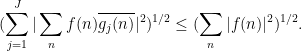
For sake of comparison, if one were to apply the Cauchy-Schwarz inequality (4) separately to each summand in (5), one would obtain the bound of , which is significantly inferior to the Bessel bound when is large. Geometrically, what is going on is this: the Cauchy-Schwarz inequality (4) is only close to sharp when and are close to parallel in the Hilbert space . But if are orthonormal, then it is not possible for any other vector to be simultaneously close to parallel to too many of these orthonormal vectors, and so the inner products of with most of the should be small. (See this previous blog post for more discussion of this principle.) One can view the Bessel inequality as formalising a repulsion principle: if correlates too much with some of the , then it does not have enough “energy” to have large correlation with the rest of the .

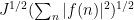
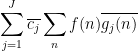
In analytic number theory applications, it is useful to generalise the Bessel inequality to the situation in which the are not necessarily orthonormal. This can be accomplished via the Cauchy-Schwarz inequality:

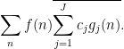
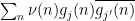
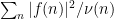
Proposition 2 (Generalised Bessel inequality) Let be finitely supported functions, and let be a non-negative function. Let be such that vanishes whenever vanishes, we have

for some sequence of complex numbers with , with the convention that vanishes whenever both vanish.

Note by relabeling that we may replace the domain here by any other at most countable set, such as the integers . (Indeed, one can give an analogue of this lemma on arbitrary measure spaces, but we will not do so here.) This result first appears in this paper of Boas.

Proof: We use the method of duality to replace the role of the function by a dual sequence . By the converse to Cauchy-Schwarz, we may write the left-hand side of (6) as

for some complex numbers with . Indeed, if all of the vanish, we can set the arbitrarily, otherwise we set to be the unit vector formed by dividing by its length. We can then rearrange this expression as

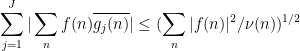
Applying Cauchy-Schwarz (dividing the first factor by and multiplying the second by , after first removing those for which vanish), this is bounded by

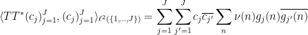
and the claim follows by expanding out the second factor.

Observe that Lemma 1 is a special case of Proposition 2 when and the are orthonormal. In general, one can expect Proposition 2 to be useful when the are almost orthogonal relative to , in that the correlations tend to be small when are distinct. In that case, one can hope for the diagonal term in the right-hand side of (6) to dominate, in which case one can obtain estimates of comparable strength to the classical Bessel inequality. The flexibility to choose different weights in the above proposition has some technical advantages; for instance, if is concentrated in a sparse set (such as the primes), it is sometimes useful to tailor to a comparable set (e.g. the almost primes) in order not to lose too much in the first factor . Also, it can be useful to choose a fairly “smooth” weight , in order to make the weighted correlations small.

Remark 3 In harmonic analysis, the use of tools such as Proposition 2 is known as the method of almost orthogonality, or the method. The explanation for the latter name is as follows. For sake of exposition, suppose that is never zero (or we remove all from the domain for which vanishes). Given a family of finitely supported functions , consider the linear operator defined by the formula

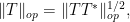
This is a bounded linear operator, and the left-hand side of (6) is nothing other than the norm of . Without any further information on the function other than its norm , the best estimate one can obtain on (6) here is clearly

where denotes the operator norm of .

The adjoint is easily computed to be

The composition of and its adjoint is then given by

From the spectral theorem (or singular value decomposition), one sees that the operator norms of and are related by the identity

and as is a self-adjoint, positive semi-definite operator, the operator norm is also the supremum of the quantity

where ranges over unit vectors in . Putting these facts together, we obtain Proposition 2; furthermore, we see from this analysis that the bound here is essentially optimal if the only information one is allowed to use about is its norm.

For further discussion of almost orthogonality methods from a harmonic analysis perspective, see Chapter VII of this text of Stein.

Exercise 4 Under the same hypotheses as Proposition 2, show that

as well as the variant inequality

Proposition 2 has many applications in analytic number theory; for instance, we will use it in later notes to control the large value of Dirichlet series such as the Riemann zeta function. One of the key benefits is that it largely eliminates the need to consider further correlations of the function (other than its self-correlation relative to , which is usually fairly easy to compute or estimate as is usually chosen to be relatively simple); this is particularly useful if is a function which is significantly more complicated to analyse than the functions . Of course, the tradeoff for this is that one now has to deal with the coefficients , which if anything are even less understood than , since literally the only thing we know about these coefficients is their square sum . However, as long as there is enough almost orthogonality between the , one can estimate the by fairly crude estimates (e.g. triangle inequality or Cauchy-Schwarz) and still get reasonably good estimates.

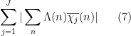
In this set of notes, we will use Proposition 2 to prove some versions of the large sieve inequality, which controls a square-sum of correlations

of an arbitrary finitely supported function with various additive characters (where ), or alternatively a square-sum of correlations

of with various primitive Dirichlet characters ; it turns out that one can prove a (slightly sub-optimal) version of this inequality quite quickly from Proposition 2 if one first prepares the sum by inserting a smooth cutoff with well-behaved Fourier transform. The large sieve inequality has many applications (as the name suggests, it has particular utility within sieve theory). For the purposes of this set of notes, though, the main application we will need it for is the Bombieri-Vinogradov theorem, which in a very rough sense gives a prime number theorem in arithmetic progressions, which, “on average”, is of strength comparable to the results provided by the Generalised Riemann Hypothesis (GRH), but has the great advantage of being unconditional (it does not require any unproven hypotheses such as GRH); it can be viewed as a significant extension of the Siegel-Walfisz theorem from Notes 2. As we shall see in later notes, the Bombieri-Vinogradov theorem is a very useful ingredient in sieve-theoretic problems involving the primes.

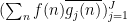
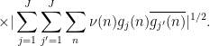
There is however one additional important trick, beyond the large sieve, which we will need in order to establish the Bombieri-Vinogradov theorem. As it turns out, after some basic manipulations (and the deployment of some multiplicative number theory, and specifically the Siegel-Walfisz theorem), the task of proving the Bombieri-Vinogradov theorem is reduced to that of getting a good estimate on sums that are roughly of the form

for some primitive Dirichlet characters . This looks like the type of sum that can be controlled by the large sieve (or by Proposition 2), except that this is an ordinary sum rather than a square sum (i.e., an norm rather than an norm). One could of course try to control such a sum in terms of the associated square-sum through the Cauchy-Schwarz inequality, but this turns out to be very wasteful (it loses a factor of about ). Instead, one should try to exploit the special structure of the von Mangoldt function , in particular the fact that it can be expressible as a Dirichlet convolution of two further arithmetic sequences (or as a finite linear combination of such Dirichlet convolutions). The reason for introducing this convolution structure is through the basic identity

for any finitely supported sequences , as can be easily seen by multiplying everything out and using the completely multiplicative nature of . (This is the multiplicative analogue of the well-known relationship between ordinary convolution and Fourier coefficients.) This factorisation, together with yet another application of the Cauchy-Schwarz inequality, lets one control (7) by square-sums of the sort that can be handled by the large sieve inequality.

As we have seen in Notes 1, the von Mangoldt function does indeed admit several factorisations into Dirichlet convolution type, such as the factorisation . One can try directly inserting this factorisation into the above strategy; it almost works, however there turns out to be a problem when considering the contribution of the portion of or that is supported at very small natural numbers, as the large sieve loses any gain over the trivial bound in such settings. Because of this, there is a need for a more sophisticated decomposition of into Dirichlet convolutions which are non-degenerate in the sense that are supported away from small values. (As a non-example, the trivial factorisation would be a totally inappropriate factorisation for this purpose.) Fortunately, it turns out that through some elementary combinatorial manipulations, some satisfactory decompositions of this type are available, such as the Vaughan identity and the Heath-Brown identity. By using one of these identities we will be able to complete the proof of the Bombieri-Vinogradov theorem. (These identities are also useful for other applications in which one wishes to control correlations between the von Mangoldt function and some other sequence; we will see some examples of this in later notes.)

For further reading on these topics, including a significantly larger number of examples of the large sieve inequality, see Chapters 7 and 17 of Iwaniec and Kowalski.

Remark 5 We caution that the presentation given in this set of notes is highly ahistorical; we are using modern streamlined proofs of results that were first obtained by more complicated arguments.

Derived multiplicative functions

Analytic number theory is often concerned with the asymptotic behaviour of various arithmetic functions: functions or from the natural numbers to the real numbers or complex numbers . In this post, we will focus on the purely algebraic properties of these functions, and for reasons that will become clear later, it will be convenient to generalise the notion of an arithmetic function to functions taking values in some abstract commutative ring . In this setting, we can add or multiply two arithmetic functions to obtain further arithmetic functions , and we can also form the Dirichlet convolution by the usual formula

Regardless of what commutative ring is in used here, we observe that Dirichlet convolution is commutative, associative, and bilinear over .

An important class of arithmetic functions in analytic number theory are the multiplicative functions, that is to say the arithmetic functions such that and

for all coprime . A subclass of these functions are the completely multiplicative functions, in which the restriction that be coprime is dropped. Basic examples of completely multiplicative functions (in the classical setting ) include

• the Kronecker delta , defined by setting for and otherwise;
• the constant function and the linear function (which by abuse of notation we denote by );
• more generally monomials for any fixed complex number (in particular, the “Archimedean characters” for any fixed ), which by abuse of notation we denote by ;
• Dirichlet characters ;
• the Liouville function ;
• the indicator function of the –smooth numbers (numbers whose prime factors are all at most ), for some given ; and
• the indicator function of the –rough numbers (numbers whose prime factors are all greater than ), for some given .

Examples of multiplicative functions that are not completely multiplicative include

• the Möbius function ;
• the divisor function (also referred to as );
• more generally, the higher order divisor functions for ;
• the Euler totient function ;
• the number of roots of a given polynomial defined over ;
• more generally, the point counting function of a given algebraic variety defined over (closely tied to the Hasse-Weil zeta function of );
• the function that counts the number of representations of as the sum of two squares;
• more generally, the function that maps a natural number to the number of ideals in a given number field of absolute norm (closely tied to the Dedekind zeta function of ).

These multiplicative functions interact well with the multiplication and convolution operations: if are multiplicative, then so are and , and if is completely multiplicative, then we also have

 

Finally, the product of completely multiplicative functions is again completely multiplicative. On the other hand, the sum of two multiplicative functions will never be multiplicative (just look at what happens at ), and the convolution of two completely multiplicative functions will usually just be multiplicative rather than completley multiplicative.

The specific multiplicative functions listed above are also related to each other by various important identities, for instance

where is an arbitrary arithmetic function.

On the other hand, analytic number theory also is very interested in certain arithmetic functions that are not exactly multiplicative (and certainly not completely multiplicative). One particularly important such function is the von Mangoldt function . This function is certainly not multiplicative, but is clearly closely related to such functions via such identities as and , where is the natural logarithm function. The purpose of this post is to point out that functions such as the von Mangoldt function lie in a class closely related to multiplicative functions, which I will call the derived multiplicative functions. More precisely:

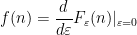
Definition 1 A derived multiplicative function is an arithmetic function that can be expressed as the formal derivative

at the origin of a family of multiplicative functions parameterised by a formal parameter . Equivalently, is a derived multiplicative function if it is the coefficient of a multiplicative function in the extension of by a nilpotent infinitesimal ; in other words, there exists an arithmetic function such that the arithmetic function is multiplicative, or equivalently that is multiplicative and one has the Leibniz rule

 

for all coprime .

More generally, for any , a -derived multiplicative function is an arithmetic function that can be expressed as the formal derivative

at the origin of a family of multiplicative functions parameterised by formal parameters . Equivalently, is the coefficient of a multiplicative function in the extension of by nilpotent infinitesimals .

We define the notion of a -derived completely multiplicative function similarly by replacing “multiplicative” with “completely multiplicative” in the above discussion.

There are Leibniz rules similar to (2) but they are harder to state; for instance, a doubly derived multiplicative function comes with singly derived multiplicative functions and a multiplicative function such that

for all coprime .

One can then check that the von Mangoldt function is a derived multiplicative function, because is multiplicative in the ring with one infinitesimal . Similarly, the logarithm function is derived completely multiplicative because is completely multiplicative in . More generally, any additive function is derived multiplicative because it is the top order coefficient of .

Remark 1 One can also phrase these concepts in terms of the formal Dirichlet series associated to an arithmetic function . A function is multiplicative if admits a (formal) Euler product; is derived multiplicative if is the (formal) first logarithmic derivative of an Euler product with respect to some parameter (not necessarily , although this is certainly an option); and so forth.

Using the definition of a -derived multiplicative function as the top order coefficient of a multiplicative function of a ring with infinitesimals, it is easy to see that the product or convolution of a -derived multiplicative function and a -derived multiplicative function is necessarily a -derived multiplicative function (again taking values in ). Thus, for instance, the higher-order von Mangoldt functions are -derived multiplicative functions, because is a -derived completely multiplicative function. More explicitly, is the top order coeffiicent of the completely multiplicative function , and is the top order coefficient of the multiplicative function , with both functions taking values in the ring of complex numbers with infinitesimals attached.

It then turns out that most (if not all) of the basic identities used by analytic number theorists concerning derived multiplicative functions, can in fact be viewed as coefficients of identities involving purely multiplicative functions, with the latter identities being provable primarily from multiplicative identities, such as (1). This phenomenon is analogous to the one in linear algebra discussed in this previous blog post, in which many of the trace identities used there are derivatives of determinant identities. For instance, the Leibniz rule

for any arithmetic functions can be viewed as the top order term in

in the ring with one infinitesimal , and then we see that the Leibniz rule is a special case (or a derivative) of (1), since is completely multiplicative. Similarly, the formulae

are top order terms of

and the variant formula is the top order term of

which can then be deduced from the previous identities by noting that the completely multiplicative function inverts multiplicatively, and also noting that annihilates . The Selberg symmetry formula

 

which plays a key role in the Erdös-Selberg elementary proof of the prime number theorem (as discussed in this previous blog post), is the top order term of the identity

involving the multiplicative functions , , , with two infinitesimals , and this identity can be proven while staying purely within the realm of multiplicative functions, by using the identities

and (1). Similarly for higher identities such as

which arise from expanding out using (1) and the above identities; we leave this as an exercise to the interested reader.

An analogous phenomenon arises for identities that are not purely multiplicative in nature due to the presence of truncations, such as the Vaughan identity

 

for any , where is the restriction of a multiplicative function to the natural numbers greater than , and similarly for , , . In this particular case, (4) is the top order coefficient of the identity

which can be easily derived from the identities and . Similarly for the Heath-Brown identity

 

valid for natural numbers up to , where and are arbitrary parameters and denotes the -fold convolution of , and discussed in this previous blog post; this is the top order coefficient of

and arises by first observing that

vanishes up to , and then expanding the left-hand side using the binomial formula and the identity .

One consequence of this phenomenon is that identities involving derived multiplicative functions tend to have a dimensional consistency property: all terms in the identity have the same order of derivation in them. For instance, all the terms in the Selberg symmetry formula (3) are doubly derived functions, all the terms in the Vaughan identity (4) or the Heath-Brown identity (5) are singly derived functions, and so forth. One can then use dimensional analysis to help ensure that one has written down a key identity involving such functions correctly, much as is done in physics.

In addition to the dimensional analysis arising from the order of derivation, there is another dimensional analysis coming from the value of multiplicative functions at primes (which is more or less equivalent to the order of pole of the Dirichlet series at ). Let us say that a multiplicative function has a pole of order if one has on the average for primes , where we will be a bit vague as to what “on the average” means as it usually does not matter in applications. Thus for instance, or has a pole of order (a simple pole), or has a pole of order (i.e. neither a zero or a pole), Dirichlet characters also have a pole of order (although this is slightly nontrivial, requiring Dirichlet’s theorem), has a pole of order (a simple zero), has a pole of order , and so forth. Note that the convolution of a multiplicative function with a pole of order with a multiplicative function with a pole of order will be a multiplicative function with a pole of order . If there is no oscillation in the primes (e.g. if for all primes , rather than on the average), it is also true that the product of a multiplicative function with a pole of order with a multiplicative function with a pole of order will be a multiplicative function with a pole of order . The situation is significantly different though in the presence of oscillation; for instance, if is a quadratic character then has a pole of order even though has a pole of order .

A -derived multiplicative function will then be said to have an underived pole of order if it is the top order coefficient of a multiplicative function with a pole of order ; in terms of Dirichlet series, this roughly means that the Dirichlet series has a pole of order at . For instance, the singly derived multiplicative function has an underived pole of order , because it is the top order coefficient of , which has a pole of order ; similarly has an underived pole of order , being the top order coefficient of . More generally, and have underived poles of order and respectively for any .

By taking top order coefficients, we then see that the convolution of a -derived multiplicative function with underived pole of order and a -derived multiplicative function with underived pole of order is a -derived multiplicative function with underived pole of order . If there is no oscillation in the primes, the product of these functions will similarly have an underived pole of order , for instance has an underived pole of order . We then have the dimensional consistency property that in any of the standard identities involving derived multiplicative functions, all terms not only have the same derived order, but also the same underived pole order. For instance, in (3), (4), (5) all terms have underived pole order (with any Mobius function terms being counterbalanced by a matching term of or ). This gives a second way to use dimensional analysis as a consistency check. For instance, any identity that involves a linear combination of and is suspect because the underived pole orders do not match (being and respectively), even though the derived orders match (both are ).

One caveat, though: this latter dimensional consistency breaks down for identities that involve infinitely many terms, such as Linnik’s identity

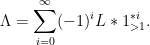
In this case, one can still rewrite things in terms of multiplicative functions as

so the former dimensional consistency is still maintained.

I thank Andrew Granville, Kannan Soundararajan, and Emmanuel Kowalski for helpful conversations on these topics.