
We will shortly turn to the complex-analytic approach to multiplicative number theory, which relies on the basic properties of complex analytic functions. In this supplement to the main notes, we quickly review the portions of complex analysis that we will be using in this course. We will not attempt a comprehensive review of this subject; for instance, we will completely neglect the conformal geometry or Riemann surface aspect of complex analysis, and we will also avoid using the various boundary convergence theorems for Taylor series or Dirichlet series (the latter type of result is traditionally utilised in multiplicative number theory, but I personally find them a little unintuitive to use, and will instead rely on a slightly different set of complex-analytic tools). We will also focus on the “local” structure of complex analytic functions, in particular adopting the philosophy that such functions behave locally like complex polynomials; the classical “global” theory of entire functions, while traditionally used in the theory of the Riemann zeta function, will be downplayed in these notes. On the other hand, we will play up the relationship between complex analysis and Fourier analysis, as we will incline to using the latter tool over the former in some of the subsequent material. (In the traditional approach to the subject, the Mellin transform is used in place of the Fourier transform, but we will not emphasise the role of the Mellin transform here.)
We begin by recalling the notion of a holomorphic function, which will later be shown to be essentially synonymous with that of a complex analytic function.
Definition 1 (Holomorphic function) Let
be an open subset of
, and let
be a function. If
, we say that
is complex differentiable at
if the limit
exists, in which case we refer to
as the (complex) derivative of
is continuous, we say that

Exercise 2 Show that a function
is continuously differentiable on
and obeys the Cauchy-Riemann equation

Basic examples of holomorphic functions include complex polynomials

as well as the complex exponential function

which are holomorphic on the entire complex plane
- (i) Establish Euler’s formula
for all
. (Hint: it is a bit tricky to do this starting from the trigonometric definitions of sine and cosine; I recommend either using the Taylor series formulations of these functions instead, or alternatively relying on the ordinary differential equations obeyed by sine and cosine.)
- (ii) Show that every non-zero complex number
such that
, and that this logarithm is unique up to integer multiples of
.
- (iii) Show that there exists a unique principal branch
of the complex logarithm in the region
, defined by requiring
and
. Show that this principal branch is holomorphic with derivative
.

In real analysis, we have the fundamental theorem of calculus, which asserts that
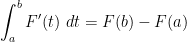
whenever ![{[a,b]}](https://s0.wp.com/latex.php?latex=%7B%5Ba%2Cb%5D%7D&bg=ffffff&fg=000000&s=0&c=20201002)
![{F: [a,b] \rightarrow {\bf R}}](https://s0.wp.com/latex.php?latex=%7BF%3A+%5Ba%2Cb%5D+%5Crightarrow+%7B%5Cbf+R%7D%7D&bg=ffffff&fg=000000&s=0&c=20201002)
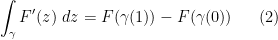
whenever 
![{\gamma: [0,1] \rightarrow \Omega}](https://s0.wp.com/latex.php?latex=%7B%5Cgamma%3A+%5B0%2C1%5D+%5Crightarrow+%5COmega%7D&bg=ffffff&fg=000000&s=0&c=20201002)


The complex fundamental theorem of calculus (2) follows easily from the real fundamental theorem and the chain rule.
In real analysis, we have the rather trivial fact that the integral of a continuous function on a closed contour is always zero:

In complex analysis, the analogous fact is significantly more powerful, and is known as Cauchy’s theorem:
Theorem 4 (Cauchy’s theorem) Let
). Then
.
Exercise 5 Use Stokes’ theorem to give a proof of Cauchy’s theorem.
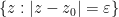
A useful reformulation of Cauchy’s theorem is that of contour shifting: if 


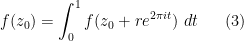
Theorem 6 (Cauchy integral formula) Let
that is traversed twice), and which encloses a bounded region
in the anticlockwise direction. Then for any
, one has

Proof: Let 


By a change of variables, the right-hand side can be expanded as

Sending 

The Cauchy integral formula has many consequences. Specialising to the case when 

whenever 
Lemma 7 (Maximum principle) Let
for all
for all
Proof: We use an argument of Landau. Fix
for some constant 


and hence

Sending 
Another basic application of the integral formula is
Corollary 8 Every holomorphic function
Conversely, it is easy to see that complex analytic functions are holomorphic. Thus, the terms “complex analytic” and “holomorphic” are synonymous, at least when working on open domains. (On a non-open set
Proof: By translation, we may suppose that 


for all 
and dominated convergence, we conclude that
with the right-hand side an absolutely convergent series for 
Exercise 9 Establish the generalised Cauchy integral formulae
for any non-negative integer
, where
is the

This in turn leads to a converse to Cauchy’s theorem, known as Morera’s theorem:
Corollary 10 (Morera’s theorem) Let
Proof: We can of course assume 


An important consequence of Morera’s theorem for us is
Corollary 11 (Locally uniform limit of holomorphic functions is holomorphic) Let
be holomorphic functions on an open set
Proof: By working locally we may assume that 
Now we study the zeroes of complex analytic functions. If a complex analytic function

for some natural number 
Recall that a rational function is a function 


Exercise 12 Show that the space of meromorphic functions on a non-empty open set
By quotienting two Taylor series, we see that if a meromorphic function

absolutely convergent in a neighbourhood of 


Exercise 13 (Residue theorem) Let
where
The residue theorem is particularly useful when applied to logarithmic derivatives 
Exercise 14 Let
), occurring at the poles and zeroes of
Remark 15 The fact that residues of logarithmic derivatives of meromorphic functions are automatically integers is a remarkable feature of the complex analytic approach to multiplicative number theory, which is difficult (though not entirely impossible) to duplicate in other approaches to the subject. Here is a sample application of this integrality, which is challenging to reproduce by non-complex-analytic means: if
as
, then
must in fact stay bounded near
is zero.
— 1. Local approximation of meromorphic functions —
Suppose 
for some non-zero constant 


as long as

again for 
In the complex approach to multiplicative number theory, it is desirable to generalise the above formulae to the case when
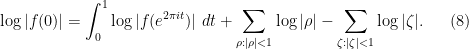
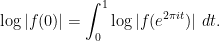
Theorem 16 (Jensen’s formula) Let
where
.

One should view (7) as a truncated (or localised) variant of (5). Note also that the summands 
Proof: By perturbing 


We may remove the poles and zeroes inside the disk 

has magnitude 


Since 


Exercise 17 (This exercise is intended for readers familiar with distribution theory, as discussed for instance in this previous blog post.) If
in the sense of distributions, where
denotes the Dirac measure at a complex number
is the distributional Laplacian
, with
denoting the real and imaginary parts of the complex variable

One application of Jensen’s formula is to control zeroes of a holomorphic function 
Exercise 18 Use Jensen’s formula to prove Liouville’s theorem: a bounded holomorphic function
for various constants
Exercise 19 Use Jensen’s formula to prove the fundamental theorem of algebra: a complex polynomial
of degree
for some complex numbers
with
. (Note that the fundamental theorem was invoked previously in this section, but only for motivational purposes, so the proof here is non-circular.)
Exercise 20 (Shifted Jensen’s formula) Let
for all
that are not zeroes or poles of
and
. (The function
appearing in the integrand is sometimes known as the Poisson kernel, particularly if one normalises so that


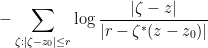
Just as (7) and (10) give truncated variants of (5), we can create truncated versions of (6). The following crude truncation is adequate for our applications:
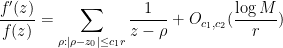
Theorem 21 (Truncated formula for log-derivative) Let
for some
and all
. Let
be constants. Then one has the approximate formula
for all
other than zeroes of
.
Proof: To abbreviate notation, we allow all implied constants in this proof to depend on 
We mimic the proof of Jensen’s formula. Firstly, we may translate and rescale so that 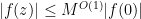

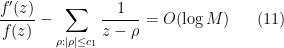
for 


on the unit circle, and so from Jensen’s formula (7) we see that

In particular we see that the number of zeroes with 

Suppose 


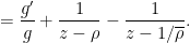
Observe from Taylor expansion that the distance between 


Similarly, given a zero 

![{t \in [0,1]}](https://s0.wp.com/latex.php?latex=%7Bt+%5Cin+%5B0%2C1%5D%7D&bg=ffffff&fg=000000&s=0&c=20201002)

and thus (by using the identity 

On the other hand, from (10) we have

which implies from (13) that 


A variant of the above argument allows one to make precise the heuristic that holomorphic functions locally look like polynomials:
Exercise 22 (Local Weierstrass factorisation) Let the notation and hypotheses be as in Theorem 21. Then show that
for all
(counting multiplicity) and
and first derivative
on this disk. Furthermore, show that the degree of

Remark 23 The classical theory of Beurling factorization of Hardy space functions on the disk into inner functions, outer functions, and Blaschke products can be viewed as a sort of limiting case of the above exercise when
; see for instance this text of Garnett for a treatment. However, we will not need this limiting theory in our applications.
— 2. The Fourier-Laplace and Fourier transforms —
There are a number of connections between complex analysis and Fourier analysis. The best known connection perhaps is between complex analytic functions on the unit disk 

Exercise 24 (Complex analysis on disk versus Fourier analysis on circle)
- Let
, and define the Fourier coefficients
for
. Show that
for all negative
(as an absolutely convergent series) in the interior
- Conversely, let
be an absolutely summable sequence of complex numbers. Show that the function
is a continuous function on the unit disk
for all
.


Remark 25 The relationship between the boundary behaviour of holomorphic functions
We will not explicitly use the above connection between complex analysis and Fourier analysis in this course (although some traces of it might be discerned in the material in the previous sections of this set of notes). Instead, we will discuss a slightly different link between the two subjects, linking complex analysis on the half-space 


Actually, for absolutely integrable 

where we extend
An application of Fubini’s theorem reveals that the integral of 


If we have a bit of smoothness on
Lemma 26 Let
be compactly supported and continuously twice differentiable. Then we have
for all
in the half-space
.

Proof: By an integration by parts, we have


since 

Corollary 27 Let
for any
. (Note from (14) that the limit exists.)
Proof: By contour shifting (using (14) to handle error terms) we see that the integral is independent of

using the principal branch of the logarithm. The integral 


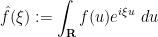
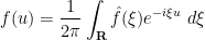
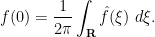
This gives a proof of one of the basic identities in Fourier analysis, the Fourier inversion formula. Given any absolutely integrable function 

(Here we use a normalisation of the Fourier transform that aligns with the traditional normalisations in complex analysis; other normalisations are used in other fields of mathematics.) We first recall some basic estimates and symmetries:
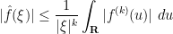
Exercise 28 (Basic estimates on Fourier transform) Let
be an integer, and let
).
- (i) Establish the pointwise bounds
for all
, where
and
.
- (ii) Suppose in addition that
extends holomorphically to the entire complex plane (with the formula (15) valid now for all
), with the pointwise bounds
for all

Exercise 29 (Basic symmetries of the Fourier transform) Let
- (i) If
for some
and all
, show that
for all
- (ii) If
for some
and all
for all
- (iii) If
for some
and all
for all
- (iv) If
for all
for all
Theorem 30 (Fourier inversion formula) Let
is bounded and absolutely integrable, and one has the inversion formula
for any
for any
, where again the integrand is absolutely integrable.

Remark 31 One can certainly relax the support and smoothness hypotheses on
Proof: From Exercise 28 with 

and so
By Exercise 29(i) we may assume without loss of generality that 
We introduce the components 
for 

From Corollary 27 we have

for either choice of sign; summing, we obtain the first claim. The second claim then follows by replacing 

Remark 32 In the above proof,
is split into a function
extending holomorphically and boundedly to the upper half-plane, and a function
extending holomorphically and boundedly to the lower half-plane. Such a decomposition solves a very simple example of the Riemann-Hilbert problem, but we will not discuss this problem further in this course.
The inversion formula gives an important identity, essentially due to Parseval and to Plancherel:
Corollary 33 (Parseval-Plancherel identities) Let
be compactly supported and continuously twice differentiable. Then we have
In particular
and

Proof: By the inversion formula we may write 

The claim then follows from Fubini’s theorem.
In the next set of notes, we will use a version of the above identity, which we will call a truncated Perron formula, to express smoothed summatory functions of arithmetic functions 
Finally, we record another important Fourier identity, the Poisson summation formula.
Theorem 34 (Poisson summation) Let
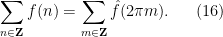
Proof: There are many ways to prove this identity, but given the spirit of this set of notes, it seems appropriate to give a complex analysis proof. By Exercise 29(i) we may assume without loss of generality that

From the Fourier inversion formula and dominated convergence again, we may rewrite this as

summing the geometric series, this becomes

Observe that the function 


and the claim then follows from one final application of dominated convergence.
There will be at least two key applications of the Poisson summation formula in this course. One is to establish the functional equation for the Riemann zeta function (as well as truncated versions of this equation, for instance involving the sum 


Exercise 35 (Good error bounds on smooth sums) Let
. Use the Poisson summation formula to show that
for all
. (This should be compared with the error term of
that one would have obtained using the methods from previous notes.) This estimate illustrates a basic principle, namely that smoother sums enjoy better asymptotics.

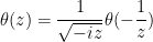
Exercise 36 (Fourier transform of Gaussian) Let
be the function defined by
for
for all
replaced by some unknown positive constant
whenever
, with the principal branch
of the complex square root, and
is the theta function
(Hint: use the Poisson summation formula and the symmetries of the Fourier transform.)


Exercise 37 (Mellin inversion formula) Let
for all
and
, where the integral is along the straight line contour from
to
. What happens when
?

Remark 38 By a simple change of variables, the above formula also leads to an inversion formula for the Mellin transform
defined for compactly supported absolutely integrable
and
, but we will not use this transform or inversion formula here.

Exercise 39 (Qualitative uncertainty principle) Let
(The exercises below should be placed earlier in this set of notes, but are at the end to avoid renumbering issues.)
Exercise 40 (Borel-Carathéodory theorem) Let
, one has
and
for all
. (Hint: there are various ways to proceed here. One is to apply Exercise 20 to
and differentiate.)


Exercise 41 (Hadamard three-lines theorem)
- (i) Let
and
be real numbers. Suppose that
such that
and
for all
for all
and
for all
and
. Use the maximum principle to verify the claim in the case that
goes to zero as
. To handle the general case, mollify
for suitable
.)
- (ii) Let
be real numbers, and let
for
and
for
for all

24 comments
Comments feed for this article
5 December, 2014 at 10:43 am
Anonymous
I think you mean 254A in the title.
[Corrected, thanks -T.]
5 December, 2014 at 11:14 am
MrCactu5 (@MonsieurCactus)
“We will not attempt a comprehensive review of this subject; for instance, we will completely neglect the conformal geometry or Riemann surface aspect of complex analysis” ;-(
5 December, 2014 at 2:27 pm
Rogier Brussee
In cor. 34, the Plancherel formula misses a hat on g.
As always, very nice notes.
[Corrected, thanks – T.]
5 December, 2014 at 10:23 pm
jlackm
Dear Professor Tao,
can one easily use Stokes’ theorem to prove Cauchy’s integral formula without assuming continuity of the partial derivatives? A priori they aren’t even Riemann integrable, and I’ve never seen this done before. This would be very nice if it’s true.
6 December, 2014 at 7:44 am
Terence Tao
Goursat’s proof of Cauchy’s theorem (and hence the integral formula) requires only complex differentiability at each point, without continuity (although when combined with Morera’s theorem, one can recover this continuity and even obtain complex analyticity). See e.g. Stein-Shakarchi http://press.princeton.edu/chapters/s02_7563.pdf . In most applications, though, whenever one establishes differentiability of a function, one also establishes continuous differentiability without much additional effort, so this additional relaxation of hypotheses is not a significant strengthening of Cauchy’s theorem in practice.
9 December, 2014 at 12:55 am
Avi Levy
In the paragraph preceeding Exercise 12, right after the definition of a meromorphic function: “which is locally to the quotient {g/h} of holomorphic functions” (I think you’re missing a word or two).
[Corrected, thanks – T.]
17 December, 2014 at 7:37 am
peteg
In the proof of Corollary 8, what allows you to switch the sum and the integral?
17 December, 2014 at 9:56 am
Terence Tao
The dominated convergence theorem (note that is uniformly bounded on the contour
  , and
, and  is bounded in magnitude by
  , which is absolutely convergent when summed in
  ). One could also use Fubini’s theorem here if desired.
27 December, 2014 at 9:00 pm
peteg
In the proof of Jensen’s formula, for the case where f has no zeros or poles in the unit disc, would a valid argument be that since log f is analytic, it satisfies the mean value property?
[Yes; this is essentially the strategy used to prove this formula in this blog post. -T.]
30 December, 2014 at 9:00 am
peteg
Can you expand on the hint for exercise 18?
3 January, 2015 at 8:54 am
Terence Tao
Suppose for instance that is not zero at the origin, but has at least one zero
  . Apply Jensen’s formula to a disk
  and obtain a contradiction for sufficiently large
  if
if  is bounded.
13 February, 2015 at 10:16 pm
254A, Notes 6: Large values of Dirichlet polynomials, zero density estimates, and primes in short intervals | What's new
[…] by exploiting the smooth nature of . Namely, by using the Poisson summation formula (Theorem 34 of Supplement 2), we can rewrite (2) […]
15 February, 2015 at 5:03 pm
254A, Notes 3: The large sieve and the Bombieri-Vinogradov theorem | What's new
[…] hence by Exercise 28 of Supplement 2, we have the […]
22 February, 2015 at 9:02 am
254A, Notes 7: Linnik’s theorem on primes in arithmetic progressions | What's new
[…] Jensen’s theorem (Theorem 16 of Supplement 2), we conclude that for any given non-principal and any , there are at most zeroes of (counting […]
1 March, 2015 at 1:13 pm
254A, Supplement 7: Normalised limit profiles of the log-magnitude of the Riemann zeta function (optional) | What's new
[…] A major topic of interest of analytic number theory is the asymptotic behaviour of the Riemann zeta function in the critical strip in the limit . For the purposes of this set of notes, it is a little simpler technically to work with the log-magnitude of the zeta function. (In principle, one can reconstruct a branch of , and hence itself, from using the Cauchy-Riemann equations, or tools such as the Borel-Carathéodory theorem, see Exercise 40 of Supplement 2.) […]
29 March, 2016 at 6:03 am
Terry Tao: 254A, Supplement 2: A little bit of complex and Fourier analysis | What’s new – Collected Links
[…] 254A, Supplement 2: A little bit of complex and Fourier analysis | What’s new n this supplement to the main notes, we quickly review the portions of complex analysis that we will be using in this course. We will not attempt a comprehensive review of this subject; for instance, we will completely neglect the conformal geometry or Riemann surface aspect of complex analysis, and we will also avoid using the various boundary convergence theorems for Taylor series or Dirichlet series (the latter type of result is traditionally utilised in multiplicative number theory, but I personally find them a little unintuitive to use, and will instead rely on a slightly different set of complex-analytic tools). We will also focus on the “local” structure of complex analytic functions, in particular adopting the philosophy that such functions behave locally like complex polynomials; the classical “global” theory of entire functions, while traditionally used in the theory of the Riemann zeta function, will be downplayed in these notes. On the other hand, we will play up […]
2 July, 2016 at 6:51 am
254A, Supplement 3: The Gamma function and the functional equation (optional) | What's new
[…] 34 from Supplement 2, at least in the case when is twice continuously differentiable and compactly supported), which […]
26 September, 2016 at 5:52 am
Anonymous
In the statement of Theorem 21, should the error term in the approximation formula for be
be  , where d is the number of zeroes of
  in the annulus
  ?
?
26 September, 2016 at 9:23 am
Terence Tao
No, because the bound (12) allows one to control the combined contribution of these zeroes, as explained in the proof.
26 September, 2016 at 9:49 pm
Anonymous
Thanks! I’ve got it now.
21 January, 2017 at 3:56 pm
254A, Notes 2: Complex-analytic multiplicative number theory | What's new
[…] come from the general theory of local factorisations of meromorphic functions, as discussed in Supplement 2; the passage from (4) to (2) is accomplished by such tools as the residue theorem and the Fourier […]
5 June, 2017 at 10:04 am
Five-Value Theorem of Nevanlinna – Elmar Klausmeier's Weblog
[…] 254A, Supplement 2: A little bit of complex and Fourier analysis, proves Poisson-Jensen formula for the logarithm of a meromorphic function in relation to its zeros within a disk […]
22 June, 2019 at 8:18 am
Helene
In Ex. 35, is it enough to assume that $N \geq 1,$ instead of $N >> 1?$
[The latter case already subsumes the former. -T]
11 October, 2021 at 9:19 am
254A, Supplement 4: Probabilistic models and heuristics for the primes (optional) | What's new
[…] 22 of Notes 2) it is a routine matter (using Proposition 16 from Notes 2 and Exercise 28 of Supplement 2) to arrive at the […]