A fundamental and recurring problem in analytic number theory is to demonstrate the presence of cancellation in an oscillating sum, a typical example of which might be a correlation
between two arithmetic functions  and
and  , which to avoid technicalities we will assume to be finitely supported (or that the
  variable is localised to a finite range, such as
  ). A key example to keep in mind for the purposes of this set of notes is the twisted von Mangoldt summatory function
that measures the correlation between the primes and a Dirichlet character  . One can get a “trivial” bound on such sums from the triangle inequality
for instance, from the triangle inequality and the prime number theorem we have

as  . But the triangle inequality is insensitive to the phase oscillations of the summands, and often we expect (e.g. from the probabilistic heuristics from Supplement 4) to be able to improve upon the trivial triangle inequality bound by a substantial amount; in the best case scenario, one typically expects a “square root cancellation” that gains a factor that is roughly the square root of the number of summands. (For instance, for Dirichlet characters of conductor
  , it is expected from probabilistic heuristics that the left-hand side of (3) should in fact be
  for any
  .)
.)
It has proven surprisingly difficult, however, to establish significant cancellation in many of the sums of interest in analytic number theory, particularly if the sums do not have a strong amount of algebraic structure (e.g. multiplicative structure) which allow for the deployment of specialised techniques (such as multiplicative number theory techniques). In fact, we are forced to rely (to an embarrassingly large extent) on (many variations of) a single basic tool to capture at least some cancellation, namely the Cauchy-Schwarz inequality. In fact, in many cases the classical case

considered by Cauchy, where at least one of  is finitely supported, suffices for applications. Roughly speaking, the Cauchy-Schwarz inequality replaces the task of estimating a cross-correlation between two different functions
  , to that of measuring self-correlations between
  and itself, or
  and itself, which are usually easier to compute (albeit at the cost of capturing less cancellation). Note that the Cauchy-Schwarz inequality requires almost no hypotheses on the functions or , making it a very widely applicable tool.
There is however some skill required to decide exactly how to deploy the Cauchy-Schwarz inequality (and in particular, how to select and ); if applied blindly, one loses all cancellation and can even end up with a worse estimate than the trivial bound. For instance, if one tries to bound (2) directly by applying Cauchy-Schwarz with the functions  and , one obtains the bound
The right-hand side may be bounded by  , but this is worse than the trivial bound (3) by a logarithmic factor. This can be “blamed” on the fact that and are concentrated on rather different sets ( is concentrated on primes, while is more or less uniformly distributed amongst the natural numbers); but even if one corrects for this (e.g. by weighting Cauchy-Schwarz with some suitable “sieve weight” that is more concentrated on primes), one still does not do any better than (3). Indeed, the Cauchy-Schwarz inequality suffers from the same key weakness as the triangle inequality: it is insensitive to the phase oscillation of the factors
  .
.
While the Cauchy-Schwarz inequality can be poor at estimating a single correlation such as (1), its power improves when considering an average (or sum, or square sum) of multiple correlations. In this set of notes, we will focus on one such situation of this type, namely that of trying to estimate a square sum
that measures the correlations of a single function with multiple other functions  . One should think of the situation in which is a “complicated” function, such as the von Mangoldt function , but the
  are relatively “simple” functions, such as Dirichlet characters. In the case when the are orthonormal functions, we of course have the classical Bessel inequality:
Lemma 1 (Bessel inequality) Let  be finitely supported functions obeying the orthonormality relationship

for all  . Then for any function , we have
For sake of comparison, if one were to apply the Cauchy-Schwarz inequality (4) separately to each summand in (5), one would obtain the bound of  , which is significantly inferior to the Bessel bound when
  is large. Geometrically, what is going on is this: the Cauchy-Schwarz inequality (4) is only close to sharp when and are close to parallel in the Hilbert space
  . But if
  are orthonormal, then it is not possible for any other vector to be simultaneously close to parallel to too many of these orthonormal vectors, and so the inner products of with most of the should be small. (See this previous blog post for more discussion of this principle.) One can view the Bessel inequality as formalising a repulsion principle: if correlates too much with some of the , then it does not have enough “energy” to have large correlation with the rest of the .
In analytic number theory applications, it is useful to generalise the Bessel inequality to the situation in which the are not necessarily orthonormal. This can be accomplished via the Cauchy-Schwarz inequality:
Proposition 2 (Generalised Bessel inequality) Let be finitely supported functions, and let  be a non-negative function. Let be such that vanishes whenever
  vanishes, we have


for some sequence  of complex numbers with
  , with the convention that
  vanishes whenever
  both vanish.
Note by relabeling that we may replace the domain  here by any other at most countable set, such as the integers
  . (Indeed, one can give an analogue of this lemma on arbitrary measure spaces, but we will not do so here.) This result first appears in this paper of Boas.
Proof: We use the method of duality to replace the role of the function by a dual sequence . By the converse to Cauchy-Schwarz, we may write the left-hand side of (6) as
for some complex numbers with . Indeed, if all of the  vanish, we can set the
  arbitrarily, otherwise we set
  to be the unit vector formed by dividing
  by its length. We can then rearrange this expression as
Applying Cauchy-Schwarz (dividing the first factor by  and multiplying the second by , after first removing those for which
  vanish), this is bounded by

and the claim follows by expanding out the second factor. 
Observe that Lemma 1 is a special case of Proposition 2 when  and the are orthonormal. In general, one can expect Proposition 2 to be useful when the are almost orthogonal relative to , in that the correlations
  tend to be small when
  are distinct. In that case, one can hope for the diagonal term
  in the right-hand side of (6) to dominate, in which case one can obtain estimates of comparable strength to the classical Bessel inequality. The flexibility to choose different weights in the above proposition has some technical advantages; for instance, if is concentrated in a sparse set (such as the primes), it is sometimes useful to tailor to a comparable set (e.g. the almost primes) in order not to lose too much in the first factor
  . Also, it can be useful to choose a fairly “smooth” weight , in order to make the weighted correlations small.
Remark 3 In harmonic analysis, the use of tools such as Proposition 2 is known as the method of almost orthogonality, or the  method. The explanation for the latter name is as follows. For sake of exposition, suppose that is never zero (or we remove all from the domain for which vanishes). Given a family of finitely supported functions , consider the linear operator
  defined by the formula
This is a bounded linear operator, and the left-hand side of (6) is nothing other than the  norm of
  . Without any further information on the function other than its
  norm
norm  , the best estimate one can obtain on (6) here is clearly

where  denotes the operator norm of
  .
.
The adjoint  is easily computed to be

The composition  of and its adjoint is then given by

From the spectral theorem (or singular value decomposition), one sees that the operator norms of and are related by the identity
and as is a self-adjoint, positive semi-definite operator, the operator norm  is also the supremum of the quantity
where  ranges over unit vectors in . Putting these facts together, we obtain Proposition 2; furthermore, we see from this analysis that the bound here is essentially optimal if the only information one is allowed to use about is its norm.
For further discussion of almost orthogonality methods from a harmonic analysis perspective, see Chapter VII of this text of Stein.
Exercise 4 Under the same hypotheses as Proposition 2, show that

as well as the variant inequality

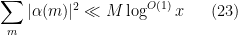
Proposition 2 has many applications in analytic number theory; for instance, we will use it in later notes to control the large value of Dirichlet series such as the Riemann zeta function. One of the key benefits is that it largely eliminates the need to consider further correlations of the function (other than its self-correlation relative to  , which is usually fairly easy to compute or estimate as is usually chosen to be relatively simple); this is particularly useful if is a function which is significantly more complicated to analyse than the functions . Of course, the tradeoff for this is that one now has to deal with the coefficients , which if anything are even less understood than , since literally the only thing we know about these coefficients is their square sum
  . However, as long as there is enough almost orthogonality between the , one can estimate the by fairly crude estimates (e.g. triangle inequality or Cauchy-Schwarz) and still get reasonably good estimates.
In this set of notes, we will use Proposition 2 to prove some versions of the large sieve inequality, which controls a square-sum of correlations

of an arbitrary finitely supported function  with various additive characters
  (where
  ), or alternatively a square-sum of correlations

of with various primitive Dirichlet characters  ; it turns out that one can prove a (slightly sub-optimal) version of this inequality quite quickly from Proposition 2 if one first prepares the sum by inserting a smooth cutoff with well-behaved Fourier transform. The large sieve inequality has many applications (as the name suggests, it has particular utility within sieve theory). For the purposes of this set of notes, though, the main application we will need it for is the Bombieri-Vinogradov theorem, which in a very rough sense gives a prime number theorem in arithmetic progressions, which, “on average”, is of strength comparable to the results provided by the Generalised Riemann Hypothesis (GRH), but has the great advantage of being unconditional (it does not require any unproven hypotheses such as GRH); it can be viewed as a significant extension of the Siegel-Walfisz theorem from Notes 2. As we shall see in later notes, the Bombieri-Vinogradov theorem is a very useful ingredient in sieve-theoretic problems involving the primes.
There is however one additional important trick, beyond the large sieve, which we will need in order to establish the Bombieri-Vinogradov theorem. As it turns out, after some basic manipulations (and the deployment of some multiplicative number theory, and specifically the Siegel-Walfisz theorem), the task of proving the Bombieri-Vinogradov theorem is reduced to that of getting a good estimate on sums that are roughly of the form
for some primitive Dirichlet characters . This looks like the type of sum that can be controlled by the large sieve (or by Proposition 2), except that this is an ordinary sum rather than a square sum (i.e., an  norm rather than an
  norm). One could of course try to control such a sum in terms of the associated square-sum through the Cauchy-Schwarz inequality, but this turns out to be very wasteful (it loses a factor of about
  ). Instead, one should try to exploit the special structure of the von Mangoldt function , in particular the fact that it can be expressible as a Dirichlet convolution
  of two further arithmetic sequences
  (or as a finite linear combination of such Dirichlet convolutions). The reason for introducing this convolution structure is through the basic identity

for any finitely supported sequences  , as can be easily seen by multiplying everything out and using the completely multiplicative nature of . (This is the multiplicative analogue of the well-known relationship
  between ordinary convolution and Fourier coefficients.) This factorisation, together with yet another application of the Cauchy-Schwarz inequality, lets one control (7) by square-sums of the sort that can be handled by the large sieve inequality.
As we have seen in Notes 1, the von Mangoldt function does indeed admit several factorisations into Dirichlet convolution type, such as the factorisation  . One can try directly inserting this factorisation into the above strategy; it almost works, however there turns out to be a problem when considering the contribution of the portion of
  or
or  that is supported at very small natural numbers, as the large sieve loses any gain over the trivial bound in such settings. Because of this, there is a need for a more sophisticated decomposition of into Dirichlet convolutions which are non-degenerate in the sense that are supported away from small values. (As a non-example, the trivial factorisation
  would be a totally inappropriate factorisation for this purpose.) Fortunately, it turns out that through some elementary combinatorial manipulations, some satisfactory decompositions of this type are available, such as the Vaughan identity and the Heath-Brown identity. By using one of these identities we will be able to complete the proof of the Bombieri-Vinogradov theorem. (These identities are also useful for other applications in which one wishes to control correlations between the von Mangoldt function and some other sequence; we will see some examples of this in later notes.)
For further reading on these topics, including a significantly larger number of examples of the large sieve inequality, see Chapters 7 and 17 of Iwaniec and Kowalski.
Remark 5 We caution that the presentation given in this set of notes is highly ahistorical; we are using modern streamlined proofs of results that were first obtained by more complicated arguments.
— 1. The large sieve inequality —
We begin with a (slightly weakened) form of the large sieve inequality for additive characters, also known as the analytic large sieve inequality, first extracted explicitly by Davenport and Halberstam from previous work on the large sieve, and then refined further by many authors (see Remark 7 below).
Proposition 6 (Analytic large sieve inequality) Let be a function supported on an interval ![{[M,M+N]}](https://s0.wp.com/latex.php?latex=%7B%5BM%2CM%2BN%5D%7D&bg=ffffff&fg=000000&s=0&c=20201002) for some
for some  and
and  , and let
  be
be  -separated (thus
  for all
  and some
  , where
  denotes the distance from
  to the nearest integer. Then

One can view this proposition as a variant of the Plancherel identity

associated to the Fourier transform on a cyclic group  . This identity also shows that apart from the implied constant, the bound (9) is essentially best possible.
Proof: By increasing  (if
(if  ) or decreasing (if
  ), we can reduce to the case
  without making the hypotheses any stronger. Thus the
  are now
  -separated, and our task is now to show that

We now wish to apply Proposition 2 (with relabeled by ), but we need to choose a suitable weight function  . It turns out that it is advantageous for technical reasons to select a weight that has good Fourier-analytic properties.
Fix a smooth non-negative function  supported on
 ![{[-1/4,1/4]}](https://s0.wp.com/latex.php?latex=%7B%5B-1%2F4%2C1%2F4%5D%7D&bg=ffffff&fg=000000&s=0&c=20201002) and not identically zero; we allow implied constants to depend on
and not identically zero; we allow implied constants to depend on  . (Actually, the smoothness of is not absolutely necessary for this argument; one could take
 ![{\psi = 1_{[-1/4,1/4]}}](https://s0.wp.com/latex.php?latex=%7B%5Cpsi+%3D+1_%7B%5B-1%2F4%2C1%2F4%5D%7D%7D&bg=ffffff&fg=000000&s=0&c=20201002) below if desired.) Consider the weight
below if desired.) Consider the weight  defined by
Observe that  for all
 ![{n \in [M,M+N]}](https://s0.wp.com/latex.php?latex=%7Bn+%5Cin+%5BM%2CM%2BN%5D%7D&bg=ffffff&fg=000000&s=0&c=20201002) . Thus, by Proposition 2 with this choice of , we reduce to showing that
. Thus, by Proposition 2 with this choice of , we reduce to showing that

whenever are complex numbers with .
We first consider the diagonal contribution . We can write in terms of the Fourier transform  of as
of as
and hence by Exercise 28 of Supplement 2, we have the bounds
(say) and thus

Thus the diagonal contribution of (10) is acceptable.
Now we consider an off-diagonal term  with
with  . By the Poisson summation formula (Theorem 34 from Supplement 2), we can rewrite this as

Now from the Fourier inversion formula, the function  has Fourier transform supported on , and so has Fourier transform supported in
 ![{[-\frac{\pi}{N}, \frac{\pi}{N}]}](https://s0.wp.com/latex.php?latex=%7B%5B-%5Cfrac%7B%5Cpi%7D%7BN%7D%2C+%5Cfrac%7B%5Cpi%7D%7BN%7D%5D%7D&bg=ffffff&fg=000000&s=0&c=20201002) . Since
. Since  is at least from the nearest integer, we conclude that
  for all integers
  , and hence all the off-diagonal terms in fact vanish! The claim follows.
Remark 7 If  are integers, one can in fact obtain the sharper bound

a result of Montgomery and Vaughan (with replaced by  , although it was observed subsequently subsequently by Paul Cohen that the additional
  term could be deleted by an amplification trick similar to those discussed in this previous post). See this survey of Montgomery for these results and on the (somewhat complicated) evolution of the large sieve, starting with the pioneering work of Linnik. However, in our applications the cruder form of the analytic large sieve inequality given by Proposition 6 will suffice.
Exercise 8 Let be a function supported on an interval . Show that for any  , one has

for all  outside of the union of
  intervals (or arcs) of length . In particular, we have
for all , and the significantly superior estimate
for most (outside of at most (say)  intervals of length ).
Exercise 9 (Continuous large sieve inequality) Let be an interval for some and , and let  be -separated.
Now we establish a variant of the analytic large sieve inequality, involving Dirichlet characters, due to Bombieri and Davenport.
Proposition 10 (Large sieve inequality for characters) Let be a function supported on an interval for some and , and let  . Then

where  denotes the sum over all primitive Dirichlet characters of modulus
  .
.
Proof: By increasing or decreasing  , we may assume that
  , so
, so  and our task is now to show that

Let be the weight from Proposition 6. By Proposition 2 (and some relabeling), using the functions  , it suffices to show that


whenever  are complex numbers with

We first establish that the diagonal contribution  to (13) is acceptable, that is to say that
The function  is the principal character of modulus ; it is periodic with period and has mean value
  . In particular, since
  , we see that
  for any interval
 ![{[M',M'+N]}](https://s0.wp.com/latex.php?latex=%7B%5BM%27%2CM%27%2BN%5D%7D&bg=ffffff&fg=000000&s=0&c=20201002) of length . From (11) and a partition into intervals of length , we see that
of length . From (11) and a partition into intervals of length , we see that

and the claim then follows from (14).
Now consider an off-diagonal term  with
with  . As
. As  are primitive, this implies that
  is a non-principal character and thus has mean zero. Let
  be the modulus of this character; by Fourier expansion we may write as a linear combination of the additive characters
  for
for  . (We can obtain explicit coefficients from this expansion by invoking Lemma 48 of Supplement 3, but we will not need those coefficients here.) Thus is a linear combination of the quantities
  for . But the modulus is the least common multiple of the moduli of , so in particular
  , while as observed in the proof of Proposition 6, we have
  whenever
  . So the off-diagonal terms all vanish, and the claim follows.
One can also derive Proposition 10 from Proposition 6:
Exercise 11 Let be a finitely supported sequence.
Remark 12 By combining the arguments in the above exercise with the results in Remark 7, one can sharpen Proposition 10 to

that is to say one can delete the implied constant. See this paper of Montgomery and Vaughan for some further refinements of this inequality.
— 2. The Barban-Davenport-Halberstam theorem —
We now apply the large sieve inequality for characters to obtain an analogous inequality for arithmetic progressions, due independently to Barban, and to Davenport and Halberstam; we state a slightly weakened form of that theorem here. For any finitely supported arithmetic function and any primitive residue class  , we introduce the discrepancy
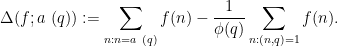
This quantity measures the extent to which is well distributed among the primitive residue classes modulo . From multiplicative Fourier inversion (see Theorem 69 from Notes 1) we have the identity

where the sum is over non-principal characters of modulus .
Theorem 13 (Barban-Davenport-Halberstam) Let  , and let be a function supported on
 ![{[1,x]}](https://s0.wp.com/latex.php?latex=%7B%5B1%2Cx%5D%7D&bg=ffffff&fg=000000&s=0&c=20201002) with the property that
with the property that

and obeying the Siegel-Walfisz property

for any fixed  , any primitive residue class
  , and any
  . Then one has
for any  , provided that
  for some sufficiently large
  depending only on
  .
.
Informally, (18) is asserting that

for “most” primitive residue classes with much smaller than  ; in most applications, the trivial bounds on
  are of the type
  , so this represents a savings of an arbitrary power of a logarithm on the average. Note that a direct application of (17) only gives (18) for of size
  ; it is the large sieve which allows for the significant enlargement of .
Proof: Let  be as above, with for some large
  to be chosen later. From (15) and the Plancherel identity one has
so our task is to show that
We cannot apply the large sieve inequality yet, because the characters here are not necessarily primitive. But we may express any non-principal character  as
as  for some primitive character
  of conductor
  , where
  are natural numbers with
  . In particular,
  and
and  . Thus we may (somewhat crudely) upper bound the left-hand side of (19) by

From Theorem 27 of Notes 1 we have  , so we may bound the above by

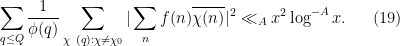
By dyadic decomposition (and adjusting slightly), it thus suffices to show that
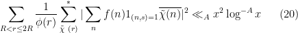
for any  and
and  .
.
From Proposition 10 and (16), we may bound the left-hand side of (20) by  . If
. If  and
and  , then we obtain (20) if is sufficiently large depending on . The only remaining case to consider is when
  . But from the Siegel-Walfisz hypothesis (17) we easily see that

for any  and any primitive character of conductor
  . Since the total number of primitive characters appearing in (20) is
  , the claim follows by taking
  large enough.
One can specialise this to the von Mangoldt function:
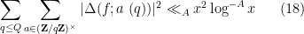
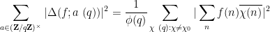
Exercise 14 Use the Barban-Davenport-Halberstam theorem and the Siegel-Walfisz theorem (Exercise 64 from Notes 2) to conclude that
![\displaystyle \sum_{q \leq Q} \sum_{a \in ({\bf Z}/q{\bf Z})^\times} |\Delta(\Lambda 1_{[1,x]}; a\ (q))|^2 \ll_A x^2 \log^{-A} x \ \ \ \ \ (21)](https://s0.wp.com/latex.php?latex=%5Cdisplaystyle++%5Csum_%7Bq+%5Cleq+Q%7D+%5Csum_%7Ba+%5Cin+%28%7B%5Cbf+Z%7D%2Fq%7B%5Cbf+Z%7D%29%5E%5Ctimes%7D+%7C%5CDelta%28%5CLambda+1_%7B%5B1%2Cx%5D%7D%3B+a%5C+%28q%29%29%7C%5E2+%5Cll_A+x%5E2+%5Clog%5E%7B-A%7D+x+%5C+%5C+%5C+%5C+%5C+%2821%29&bg=ffffff&fg=000000&s=0&c=20201002)
for any , provided that for some sufficiently large depending only on . Obtain a similar claim with replaced by the Möbius function.
Remark 15 Recall that the implied constants in the Siegel-Walfisz theorem depended on in an ineffective fashion. As such, the implied constants in (21) also depend ineffectively on . However, if one replaces Siegel’s theorem by an effective substitute such as Tatuzawa’s theorem (see Theorem 62 of Notes 2) or the Landau-Page theorem (Theorem 53 of Notes 2), one can obtain an effective version of the Siegel-Walfisz theorem for all moduli that are not multiples of a single exceptional modulus  . One can then obtain an effective version of (21) if one restricts to moduli that are not multiples of . Similarly for the Bombieri-Vinogradov theorem in the next section. Such variants of the Barban-Davenport-Halberstam theorem or Bombieri-Vinogradov theorem can be used as a substitute in some applications to remove any ineffective dependence of constants, at the cost of making the argument slightly more convoluted.
— 3. The Bombieri-Vinogradov theorem —
The Barban-Davenport-Halberstam theorem controls the discrepancy after averaging in both the modulus and the residue class  . For many problems in sieve theory, it turns out to be more important to control the discrepancy with an averaging only in the modulus , with the residue class being allowed to vary in in the “worst-case” fashion. Specifically, one often wishes to control expressions of the form

for some finitely supported and  . This expression is difficult to control for arbitrary , but it turns out that one can obtain a good bound if is expressible as a Dirichlet convolution
  for some suitably “non-degenerate” sequences . More precisely, we have the following general form of the Bombieri-Vinogradov theorem, first articulated by Motohashi:
Theorem 16 (General Bombieri-Vinogradov theorem) Let , let  be such that
  , and let be arithmetic functions supported on
 ![{[1,M]}](https://s0.wp.com/latex.php?latex=%7B%5B1%2CM%5D%7D&bg=ffffff&fg=000000&s=0&c=20201002) ,
, ![{[1,N]}](https://s0.wp.com/latex.php?latex=%7B%5B1%2CN%5D%7D&bg=ffffff&fg=000000&s=0&c=20201002) respectively, with
respectively, with
and
Suppose that  obeys the Siegel-Walfisz property

for all , all primitive residue classes , and all . Then one has

for any , provided that  and
and  for some sufficiently large depending on .
Proof: We adapt the arguments of the previous section. From (15) and the triangle inequality, we have

and so we can upper bound the left-hand side of (26) by

As in the previous section, we may reduce to primitive characters and bound this expression by

By dyadic decomposition (and adjusting slightly), it thus suffices to show that
for all and , and any  , assuming and with sufficiently large depending on .
We cannot yet easily apply the large sieve inequality, because the character sums here are not squared. But we now crucially exploit the Dirichlet convolution structure using the identity (8), to factor  as the product of
  and
and  . From the Cauchy-Schwarz inequality, we may thus bound (27) by the geometric mean of
and

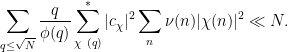
Now we have the all-important square needed in the large sieve inequality. From (23), (24) and Proposition 2, we may bound (28) by
and (29) by
and so (27) is bounded by

Since  , we can write this as

Since  and
and  , we obtain (27) if and is sufficiently large depending on . The only remaining case to handle is when
  . In this case, we can use the Siegel-Walfisz hypothesis (25) as in the previous section to bound (29) by
  for any
  . Meanwhile, from (30), (28) is bounded by
  . By taking sufficiently large, we conclude (27) in this case also.
In analogy with Exercise 14, we would like to apply this general result to specific arithmetic functions, such as the von Mangoldt function or the Möbius function , and in particular to prove the following famous result of Bombieri and of A. I. Vinogradov (not to be confused with the more well known number theorist I. M. Vinogradov):
Theorem 17 (Bombieri-Vinogradov theorem) Let  . Then one has
![\displaystyle \sum_{q \leq Q} \sup_{a \in ({\bf Z}/q{\bf Z})^\times} |\Delta(\Lambda 1_{[1,x]}; a\ (q))| \ll_{A} x \log^{-A} x \ \ \ \ \ (31)](https://s0.wp.com/latex.php?latex=%5Cdisplaystyle++%5Csum_%7Bq+%5Cleq+Q%7D+%5Csup_%7Ba+%5Cin+%28%7B%5Cbf+Z%7D%2Fq%7B%5Cbf+Z%7D%29%5E%5Ctimes%7D+%7C%5CDelta%28%5CLambda+1_%7B%5B1%2Cx%5D%7D%3B+a%5C+%28q%29%29%7C+%5Cll_%7BA%7D+x+%5Clog%5E%7B-A%7D+x+%5C+%5C+%5C+%5C+%5C+%2831%29&bg=ffffff&fg=000000&s=0&c=20201002)
for any , provided that for some sufficiently large depending on .
Informally speaking, the Bombieri-Vinogradov theorem asserts that for “almost all” moduli that are significantly less than  , one has
![\displaystyle |\Delta(\Lambda 1_{[1,x]}; a\ (q))| \ll_A \frac{x}{\phi(q)} \log^{-A} x](https://s0.wp.com/latex.php?latex=%5Cdisplaystyle++%7C%5CDelta%28%5CLambda+1_%7B%5B1%2Cx%5D%7D%3B+a%5C+%28q%29%29%7C+%5Cll_A+%5Cfrac%7Bx%7D%7B%5Cphi%28q%29%7D+%5Clog%5E%7B-A%7D+x&bg=ffffff&fg=000000&s=0&c=20201002)
for all primitive residue classes to this modulus. This should be compared with the Generalised Riemann Hypothesis (GRH), which gives the bound
![\displaystyle |\Delta(\Lambda 1_{[1,x]}; a\ (q))| \ll x^{1/2} \log^2 x](https://s0.wp.com/latex.php?latex=%5Cdisplaystyle++%7C%5CDelta%28%5CLambda+1_%7B%5B1%2Cx%5D%7D%3B+a%5C+%28q%29%29%7C+%5Cll+x%5E%7B1%2F2%7D+%5Clog%5E2+x+&bg=ffffff&fg=000000&s=0&c=20201002)
for all  ; see Exercise 48 of Notes 2. Thus one can view the Bombieri-Vinogradov theorem as an assertion that the GRH holds (with a slightly weaker error term) “on average”, at least insofar as the impact of GRH on the prime number theorem in arithmetic progressions is concerned.
The initial arguments of Bombieri and Vinogradov were somewhat complicated, in particular involving the explicit formula for -functions (Exercise 45 of Notes 2); the modern proof of the Bombieri-Vinogradov theorem avoids this and proceeds instead through Theorem 16 (or a close cousin thereof). Note that this theorem generalises the Siegel-Walfisz theorem (Exercise 64 of Notes 2), which is equivalent to the special case of Theorem 17 when  .
.
The obvious thing to try when proving Theorem 17 using Theorem 16 is to use one of the basic factorisations of such functions into Dirichlet convolutions, e.g. , and then to decompose that convolution into pieces  of the form required in Theorem 16; we will refer to such convolutions as Type II convolutions, loosely following the terminology of Vaughan. However, one runs into a problem coming from the components of the factors
  supported at small numbers (of size
  ), as the parameters associated to those parameters cannot obey the conditions ,
  . Indeed, observe that any Type II convolution will necessarily vanish at primes of size comparable to , and so one cannot possibly represent functions such as or purely in terms of such Type II convolutions.
However, it turns out that we can still decompose functions such as  into two types of convolutions: not just the Type II convolutions considered above, but also a further class of Type I convolutions , in which one of the factors, say , is very slowly varying (or “smooth”) and supported on a very long interval, e.g.
 ![{\beta = 1_{[N,2N]}}](https://s0.wp.com/latex.php?latex=%7B%5Cbeta+%3D+1_%7B%5BN%2C2N%5D%7D%7D&bg=ffffff&fg=000000&s=0&c=20201002) for some large ; with these sums
for some large ; with these sums  is permitted to be concentrated arbitrarily close to
  , and in particular the Type I convolution can be non-zero on primes comparable to . It turns out that bounding the discrepancy of Type I convolutions is relatively easy, and leads to a proof of Theorem 17.
We turn to the details. There are a number of decompositions of or that one could use to accomplish the desired task. One popular choice of decomposition is the Vaughan identity, which may be compared with the decompositions appearing in the Dirichlet hyperbola method (see Section 3 of Notes 1):
Lemma 18 (Vaughan identity) For any  , one has

where  ,
,  ,
,  , and
, and  .
.
In this decomposition,  and
and  are typically two small powers of (e.g.
  ), although the exact choice of
  is often not of critical importance. The terms
  and
and  are “Type I” convolutions, the terms
  should be considered as “Type II” convolutions. The term
  is a lower order error that is usually disposed of quite quickly. The Vaughan identity is already strong enough for many applications, but in some more advanced applications (particularly those in which one exploits the structure of triple or higher convolutions) it becomes convenient to use more sophisticated identities such as the Heath-Brown identity, which we will discuss in later notes.
Proof: Since  and
and  , we have

Convolving both sides by  and using the identities
  and
and  , we obtain the claim.
Armed with this identity and Proposition 2 we may now finish off the proof of the Bombieri-Vinogradov theorem. We may assume that is large (depending on ) as the claim is trivial otherwise. We apply the Vaughan identity (32) with (actually for our argument below, any choice of with  and
and  would have sufficed). By the triangle inequality, it now suffices to establish (31) with replaced by , ,
  , and
, and  .
.
The term is easily disposed of: from the triangle inequality (and crudely bounding by  ) we see that
![\displaystyle \Delta( \Lambda_{\leq V} 1_{[1,x]}; a\ (q)) \ll \frac{V}{\phi(q)} \log x](https://s0.wp.com/latex.php?latex=%5Cdisplaystyle++%5CDelta%28+%5CLambda_%7B%5Cleq+V%7D+1_%7B%5B1%2Cx%5D%7D%3B+a%5C+%28q%29%29+%5Cll+%5Cfrac%7BV%7D%7B%5Cphi%28q%29%7D+%5Clog+x&bg=ffffff&fg=000000&s=0&c=20201002)
and the claim follows since  and
and  .
.
Next, we deal with the Type II convolution  . The presence of the
 ![{1_{[1,x]}}](https://s0.wp.com/latex.php?latex=%7B1_%7B%5B1%2Cx%5D%7D%7D&bg=ffffff&fg=000000&s=0&c=20201002) cutoff is slightly annoying (it prevents one from directly applying Proposition 2), but we will deal with this by using the following finer-than-dyadic decomposition trick, originally due to Fouvry and to Fouvry-Iwaniec. We may replace
cutoff is slightly annoying (it prevents one from directly applying Proposition 2), but we will deal with this by using the following finer-than-dyadic decomposition trick, originally due to Fouvry and to Fouvry-Iwaniec. We may replace  by
by ![{(\mu_{>U}*1) 1_{(U,x]}}](https://s0.wp.com/latex.php?latex=%7B%28%5Cmu_%7B%3EU%7D%2A1%29+1_%7B%28U%2Cx%5D%7D%7D&bg=ffffff&fg=000000&s=0&c=20201002) , since the portion of
, since the portion of  on
on  has no contribution. We may similarly replace
  by
by ![{\Lambda 1_{(V,x]}}](https://s0.wp.com/latex.php?latex=%7B%5CLambda+1_%7B%28V%2Cx%5D%7D%7D&bg=ffffff&fg=000000&s=0&c=20201002) . Next, we set
. Next, we set  , and decompose into
  components , each of which is supported in an interval
 ![{[M, \lambda M]}](https://s0.wp.com/latex.php?latex=%7B%5BM%2C+%5Clambda+M%5D%7D&bg=ffffff&fg=000000&s=0&c=20201002) and bounded in magnitude by
and bounded in magnitude by  for some
  . We similarly decompose into components supported in an interval
 ![{[N, \lambda N]}](https://s0.wp.com/latex.php?latex=%7B%5BN%2C+%5Clambda+N%5D%7D&bg=ffffff&fg=000000&s=0&c=20201002) and bounded in magnitude by
and bounded in magnitude by  for some
  . Thus
 ![{(\mu_{>U} * \Lambda_{>V} * 1) 1_{[1,x]}}](https://s0.wp.com/latex.php?latex=%7B%28%5Cmu_%7B%3EU%7D+%2A+%5CLambda_%7B%3EV%7D+%2A+1%29+1_%7B%5B1%2Cx%5D%7D%7D&bg=ffffff&fg=000000&s=0&c=20201002) can be decomposed into
can be decomposed into  terms of the form
 ![{(\alpha*\beta)1_{[1,x]}}](https://s0.wp.com/latex.php?latex=%7B%28%5Calpha%2A%5Cbeta%291_%7B%5B1%2Cx%5D%7D%7D&bg=ffffff&fg=000000&s=0&c=20201002) for various that are components of and respectively.
for various that are components of and respectively.
If  then vanishes, so we may assume that . By construction we also have
  , so in particular if depends only on (recall we are assuming to be large). If
  , then
 ![{(\alpha*\beta)1_{[1,x]} = \alpha*\beta}](https://s0.wp.com/latex.php?latex=%7B%28%5Calpha%2A%5Cbeta%291_%7B%5B1%2Cx%5D%7D+%3D+%5Calpha%2A%5Cbeta%7D&bg=ffffff&fg=000000&s=0&c=20201002) . The bounds (23), (24) are clear (bounding in magnitude by ), and from the Siegel-Walfisz theorem we see that the components obey the hypothesis (25). Thus by applying Proposition 2 (with replaced by
. The bounds (23), (24) are clear (bounding in magnitude by ), and from the Siegel-Walfisz theorem we see that the components obey the hypothesis (25). Thus by applying Proposition 2 (with replaced by  ) we see that the total contribution of all the terms with is acceptable.
It remains to control the total contribution of the terms with  . Note that for each there are only
  choices of that are in this range, so there are only
  such terms to deal with. We then crudely bound
![\displaystyle \sup_{a \in ({\bf Z}/q{\bf Z})^\times} \Delta( \alpha*\beta 1_{[1,x]}; a\ (q) ) \ll \sup_{a \in ({\bf Z}/q{\bf Z})^\times} \sum_{n = a\ (q)} |\alpha| * |\beta|(n)](https://s0.wp.com/latex.php?latex=%5Cdisplaystyle++%5Csup_%7Ba+%5Cin+%28%7B%5Cbf+Z%7D%2Fq%7B%5Cbf+Z%7D%29%5E%5Ctimes%7D+%5CDelta%28+%5Calpha%2A%5Cbeta+1_%7B%5B1%2Cx%5D%7D%3B+a%5C+%28q%29+%29+%5Cll+%5Csup_%7Ba+%5Cin+%28%7B%5Cbf+Z%7D%2Fq%7B%5Cbf+Z%7D%29%5E%5Ctimes%7D+%5Csum_%7Bn+%3D+a%5C+%28q%29%7D+%7C%5Calpha%7C+%2A+%7C%5Cbeta%7C%28n%29&bg=ffffff&fg=000000&s=0&c=20201002)

Since  and , one has either
  or
or  . If , we observe that for each fixed in the above sum, there are
  choices of that contribute, so the double sum is
  (using the mean value bounds for ). Thus we see that the total contribution of this case is at most
which is acceptable.
Now we consider the case when . For fixed in the above sum, the sum in can be bounded by  , thanks to Corollary 26 below (taking, say,
  and
and  ). The total contribution of this sum is then

which is also acceptable.
Now let us consider a Type I term  . From the triangle inequality have
![\displaystyle |\Delta((\mu_{\leq U} * L) 1_{[1,x]}; a\ (q))| \leq \sum_{d: (d,q)=1} |\mu_{\leq U}(d)| |\Delta( L 1_{[1,x/d]}; a/d\ (q) )|.](https://s0.wp.com/latex.php?latex=%5Cdisplaystyle++%7C%5CDelta%28%28%5Cmu_%7B%5Cleq+U%7D+%2A+L%29+1_%7B%5B1%2Cx%5D%7D%3B+a%5C+%28q%29%29%7C+%5Cleq+%5Csum_%7Bd%3A+%28d%2Cq%29%3D1%7D+%7C%5Cmu_%7B%5Cleq+U%7D%28d%29%7C+%7C%5CDelta%28+L+1_%7B%5B1%2Cx%2Fd%5D%7D%3B+a%2Fd%5C+%28q%29+%29%7C.&bg=ffffff&fg=000000&s=0&c=20201002)
We exploit the monotonicity of via the following simple fact:
Exercise 19 Let ![{f: [y,x] \rightarrow {\bf R}}](https://s0.wp.com/latex.php?latex=%7Bf%3A+%5By%2Cx%5D+%5Crightarrow+%7B%5Cbf+R%7D%7D&bg=ffffff&fg=000000&s=0&c=20201002) be a monotone function. Show that
be a monotone function. Show that
![\displaystyle |\Delta( f 1_{[y,x]}; a\ (q) )| \ll |f(y)| + |f(x)|](https://s0.wp.com/latex.php?latex=%5Cdisplaystyle++%7C%5CDelta%28+f+1_%7B%5By%2Cx%5D%7D%3B+a%5C+%28q%29+%29%7C+%5Cll+%7Cf%28y%29%7C+%2B+%7Cf%28x%29%7C&bg=ffffff&fg=000000&s=0&c=20201002)
for all primitive residue classes . (Hint: use Lemma 2 from Notes 1 and a change of variables.)
Applying this exercise, we see that the contribution of this term to (31) is  , which is acceptable since
  and
and  .
.
A similar argument for the Type I term term (with  and replacing
  and ) gives a contribution to (31) of


which is also acceptable since and . This concludes the proof of Theorem 17.
Exercise 20 Strengthen the Bombieri-Vinogradov theorem by showing that
![\displaystyle \sum_{q \leq Q} \sup_{y \leq x} \sup_{a \in ({\bf Z}/q{\bf Z})^\times} |\Delta(\Lambda 1_{[1,y]}; a\ (q))| \ll_{A} x \log^{-A} x](https://s0.wp.com/latex.php?latex=%5Cdisplaystyle++%5Csum_%7Bq+%5Cleq+Q%7D+%5Csup_%7By+%5Cleq+x%7D+%5Csup_%7Ba+%5Cin+%28%7B%5Cbf+Z%7D%2Fq%7B%5Cbf+Z%7D%29%5E%5Ctimes%7D+%7C%5CDelta%28%5CLambda+1_%7B%5B1%2Cy%5D%7D%3B+a%5C+%28q%29%29%7C+%5Cll_%7BA%7D+x+%5Clog%5E%7B-A%7D+x+&bg=ffffff&fg=000000&s=0&c=20201002)
for all and , if for some sufficiently large depending on . (Hint: at present  ranges over an uncountable number of values, but if one can round to the nearest multiple of (say)
  then there are only
  values of in the supremum that need to be considered. Then use the original Bombieri-Vinogradov theorem as a black box.)
Exercise 21 For any  , establish the Vaughan-type identity

and use this to show that the Bombieri-Vinogradov theorem continues to hold when is replaced by .
Exercise 22 Let us say that  is a level of distribution for the von Mangoldt function if one has
![\displaystyle \sum_{q \leq Q} \sup_{a \in ({\bf Z}/q{\bf Z})^\times} |\Delta(\Lambda 1_{[1,x]}; a\ (q))| \ll_{A,\theta} x \log^{-A} x](https://s0.wp.com/latex.php?latex=%5Cdisplaystyle++%5Csum_%7Bq+%5Cleq+Q%7D+%5Csup_%7Ba+%5Cin+%28%7B%5Cbf+Z%7D%2Fq%7B%5Cbf+Z%7D%29%5E%5Ctimes%7D+%7C%5CDelta%28%5CLambda+1_%7B%5B1%2Cx%5D%7D%3B+a%5C+%28q%29%29%7C+%5Cll_%7BA%2C%5Ctheta%7D+x+%5Clog%5E%7B-A%7D+x+&bg=ffffff&fg=000000&s=0&c=20201002)
whenever and  ; thus, for instance, the Bombieri-Vinogradov theorem implies that every
  is a level of distribution for . Use the Cramér random model (see Section 1 of Supplement 4) to predict that every is a level of distribution for ; this claim is known as the Elliott-Halberstam conjecture, and would have a number of consequences in sieve theory. Unfortunately, no level of distribution above
  (or even at ) is currently known, however there are weaker versions of the Elliott-Halberstam conjecture known with levels above which do have some interesting number-theoretic consequences; we will return to this point in later notes. For now, we will just remark that appears to be the limit of what one can do by using the large sieve and Dirichlet character methods in this set of notes, and all the advances beyond have had to rely on other tools (such as exponential sum estimates), although the Cauchy-Schwarz inequality remains an indispensable tool in all of these results.
Exercise 23 Strengthen the Bombieri-Vinogradov theorem by showing that
![\displaystyle \sum_{q \leq Q} \tau(q)^C \sup_{a \in ({\bf Z}/q{\bf Z})^\times} |\Delta(\Lambda 1_{[1,x]}; a\ (q))| \ll_{A,C} x \log^{-A} x](https://s0.wp.com/latex.php?latex=%5Cdisplaystyle++%5Csum_%7Bq+%5Cleq+Q%7D+%5Ctau%28q%29%5EC+%5Csup_%7Ba+%5Cin+%28%7B%5Cbf+Z%7D%2Fq%7B%5Cbf+Z%7D%29%5E%5Ctimes%7D+%7C%5CDelta%28%5CLambda+1_%7B%5B1%2Cx%5D%7D%3B+a%5C+%28q%29%29%7C+%5Cll_%7BA%2CC%7D+x+%5Clog%5E%7B-A%7D+x+&bg=ffffff&fg=000000&s=0&c=20201002)
for all ,  , and , if for some sufficiently large depending on
  . (Hint: use the Cauchy-Schwarz inequality and the trivial bound
 ![{|\Delta(\Lambda 1_{[1,x]}; a\ (q))| \ll \frac{x}{q} \log x}](https://s0.wp.com/latex.php?latex=%7B%7C%5CDelta%28%5CLambda+1_%7B%5B1%2Cx%5D%7D%3B+a%5C+%28q%29%29%7C+%5Cll+%5Cfrac%7Bx%7D%7Bq%7D+%5Clog+x%7D&bg=ffffff&fg=000000&s=0&c=20201002) , together with elementary estimates on such sums as
, together with elementary estimates on such sums as  .)
.)
Exercise 24 Show that the Bombieri-Vinogradov theorem continues to hold if the von Mangoldt function is replaced by the indicator function  of the primes.
— 4. Appendix: the divisor function in arithmetic progressions —
We begin with a lemma of Landreau that controls the divisor function by a short divisor sum.
Lemma 25 For any  one has

for all natural numbers .
Proof: We write  , where is the product of all the prime factors of that are greater than or equal to
  , and is the product of all the prime factors of that are less than , counting multiplicity of course. By a greedy algorithm, we can repeatedly pull out factors of of size between and
  until the remaining portion of falls below , yielding a factorisation of the form
  where
where  lie between and ,
  is at most , and (if )
  is at least . The lower bounds on
  and imply that
  . By the trivial inequality
  we have

and thus by the pigeonhole principle one has

for some  . Since
  is a factor of that is at most , this gives the claim as long as . If
  , then as each of the are at least , we see that
  and cannot exceed . If we now use the inequality

and repeat the pigeonholing argument, we again obtain the claim.
Corollary 26 Let  , let
, let  , let
, let  , and let be a primitive residue class with
  . Then

One can lower the exponent of the logarithm here to (consistent with the heuristic that the average value of  for
for  is
is  ), but this requires additional arguments; see for instance this previous blog post. In contrast, the divisor bound
  only gives an upper bound of
  here.
here.
Proof: We allow implied constants to depend on  . Set
. Set  . Using Lemma 25 we have
for all  , and so the left-hand side of (33) is bounded by
The conditions  ,
,  constrain to either the empty set, or an arithmetic progression of modulus
  , so the inner sum is
  . On the other hand, from Theorem 27 (or Exercise 29) of Notes 1 we have

and the claim follows.
Exercise 27 Under the same assumptions as in Corollary 26, establish the bound

for any  .
.

to
used to prove Proposition 6.)
, show that

is the set of congruence classes
is the sum over all characters (not necessarily primitive) of modulus


25 comments
Comments feed for this article
10 January, 2015 at 3:39 pm
Anonymous
These methodologies are too complicated to reach the problems for which they are devised. It detracts attention from the fundamental underlying structure of the integers and primes.
15 January, 2015 at 3:12 am
Sayan Chattopadhyay
Sir can u please tell me that has the Riemann Hypothesis been proven by someone.
16 January, 2015 at 2:42 am
Anonymous
It seems that in order to apply proposition 2, the almost orthogonality condition on the functions is quite restrictive (e.g. to be exponentials or characters – for which the non-diagonal contribution can be efficiently estimated.)
16 January, 2015 at 9:40 am
Terence Tao
Yes, the in practice have to be somewhat structured, but this still gives quite a wide range of applicability since
  remains completely arbitrary. For instance, if one takes
  then one will be able to bound the number of places where Dirichlet series (with arbitrary coefficients) are large, which, among other things, can be used to establish zero density estimates for the zeta function; similarly if one takes
  then one can obtain zero density estimates for Dirichlet L-functions. (This will be discussed in later notes.) There are also more sophisticated structured functions than exponential phases or Dirichlet characters that one can compute correlations of using more advanced methods; for instance, “trace weights” that arise from traces of Frobenius on a suitable sheaf can be controlled using Deligne’s work on the Riemann hypothesis for varieties and sheaves, which allows one to take
  to be an exponential sum such as a Kloosterman sum. (Automorphic forms and homogeneous dynamics are two other sources of non-trivial cancellation that can be exploited in some number-theoretic situations.)
One can also interpret Linnik’s dispersion method as a type of application of Proposition 2 in which the functions are not so completely structured that their correlations can be read off right away, but their correlations are at least simpler to estimate than the original correlations
  , and one may need to perform some further application of Cauchy-Schwarz or similar tools to get enough control on the former correlations to arrive at control of the latter. (The proof of the equidistribution estimates Zhang used to establish bounded gaps between primes is a good example of this sort of technique.)
16 January, 2015 at 2:49 pm
Kyle Pratt
I am slightly confused about the treatment of the Type II convolution in the proof of Bombieri-Vinogradov. From Vaughan’s identity we have , but you wrote
  . Is this just a typo, or is there an easy way to deal with the
  ?
?
[Oops, this was indeed a typo; I’ve folded the 1 into the Mobius factor now. -T.]
16 January, 2015 at 4:44 pm
Mike_Miller
Dear Professor Tao. Forgive me but this doesn’t make sense.
17 January, 2015 at 3:05 am
Anonymous
Is it possible to increase the exponent in theorem 17 by taking the supremun in (31) over “typical
  ” or “almost every
  ” in some sense?
[Yes; see Theorem 13. -T.]
20 January, 2015 at 3:19 pm
Kyle Pratt
I think there is an error in the equation after “We then crudely bound…” The second seems to rely on the assumption that
  . This is not true since (as is pointed out in the paragraph before the problematic equation)
  , so really
  is bounded in magnitude by
  . I haven’t checked carefully, but this probably just adds some extra logs to the final result, and these will be harmless.
[Corrected, thanks – T.]
21 January, 2015 at 10:50 am
MrCactu5 (@MonsieurCactus)
I am struggling to follow your FAQ on the primes, but I notice you don’t say much about van Mangoldt until the very very end.
It seems fair to say Bombieri-Vinogradov is a step towards the Generalized Riemann hypothesis, giving very detailed information about the distribution of primes on arithmetic sequences.
13 February, 2015 at 10:16 pm
254A, Notes 6: Large values of Dirichlet polynomials, zero density estimates, and primes in short intervals | What's new
[…] for Dirichlet series. Our approach to these theorems will follow the same sort of methods used in Notes 3, in particular relying on the generalised Bessel inequality from those […]
18 February, 2015 at 1:51 pm
254A, Notes 4: Some sieve theory | What's new
[…] von Mangoldt function ), then estimates such as the Bombieri-Vinogradov theorem, Theorem 17 from Notes 3, turn out to be particularly useful in this regard; in other contexts, the required […]
22 February, 2015 at 9:02 am
254A, Notes 7: Linnik’s theorem on primes in arithmetic progressions | What's new
[…] use the generalised Bessel inequality (Proposition 2 from Notes 3) with to conclude […]
30 March, 2015 at 12:50 pm
254A, Notes 8: The Hardy-Littlewood circle method and Vinogradov’s theorem | What's new
[…] that in the proof of the Bombieri-Vinogradov theorem (see Notes 3), sums such as or were handled by using combinatorial identities such as Vaughan’s identity […]
10 April, 2015 at 10:02 am
254A, Supplement 5: The linear sieve and Chen’s theorem (optional) | What's new
[…] is the multiplicative function with and for . From the Bombieri-Vinogradov theorem (Theorem 17 of Notes 3) we […]
17 November, 2015 at 8:42 am
Klaus Roth | What's new
[…] the clean and general almost orthogonality principle that we have today (discussed for instance in these lecture notes of mine). The paper of Roth that had the most impact on my own personal work was his three-page paper […]
4 January, 2019 at 10:24 am
Spacing of Quadratic Fractions | George Shakan
[…] is the Von Mongoldt function. They use Vaughan’s identity on to decompose (3) into Type I and Type II sums for the […]
20 June, 2019 at 10:28 am
Maths student
Dear Prof. Tao,
in the proof of the large sieve inequality, you talk about “increasing N or decreasing Q”. That’s a little informal, and this kind of language continues to itch underneath my fingernails.
I should be most pleased if this could be changed.
By the way: Will these notes be transformed into a book? It would be much appreciated!
20 June, 2019 at 11:36 am
Anonymous
That is barely informal. If *that* bothers you so much, you shouldn’t be reading these notes.
12 November, 2019 at 6:47 pm
254A, Notes 9 – second moment and entropy methods | What's new
[…] To get a feel for this inequality, suppose for sake of discussion that and all have unit variance and , but that the are pairwise uncorrelated. Then the right-hand side is equal to , and the left-hand side is the sum of squares of the correlations between and each of the . Any individual correlation is then still permitted to be as large as , but it is not possible for multiple correlations to be this large simultaneously. This is geometrically intuitive if one views the random variables as vectors in a Hilbert space (and correlation as a rough proxy for the angle between such vectors). This lemma also shares many commonalities with the large sieve inequality, discussed in this set of notes. […]
4 November, 2020 at 10:34 am
Noam
I think that the bound on the LHS in the first inequality of exercise 4 is not optimal, if I’m not wrong using cauchy’s inequality term wise yields a better result (leaving only diagonal terms terms j=j’).
[This is incorrect. Note there is no summation in the first factor on the RHS. -T]
20 March, 2022 at 1:46 pm
Quân Nguyễn
Dear professor Tao, or a constant would satisfy all the conditions in the Generalized Bessel’s inequality though the attempt is only valid for
  by using
 ![\frac{2}{\pi} x \leq \sin x, x \in [0, \pi / 2 ]](https://s0.wp.com/latex.php?latex=%5Cfrac%7B2%7D%7B%5Cpi%7D+x+%5Cleq+%5Csin+x%2C+x+%5Cin+%5B0%2C+%5Cpi+%2F+2+%5D+&bg=ffffff&fg=545454&s=0&c=20201002) .
.
I did try an attempt of proving Analytic large sieve inequality by myself and found out that it seems that the choice for
20 March, 2022 at 3:10 pm
Quân Nguyễn
I also do have one more inquiry in the proof of BDH theorem, so the same as in displayed proof, we will start at:
and indeed, one needs to show that:
for all
where . Then since the function
  is supported on
 ![[1,x]](https://s0.wp.com/latex.php?latex=%5B1%2Cx%5D&bg=ffffff&fg=545454&s=0&c=20201002) , and so by Large sieve inequality for characters, one obtains:
, and so by Large sieve inequality for characters, one obtains:
which holds for all where
where  depends on
  . My apology if it's an obvious error but the attempt does not show the use of the Siegel-Walfisz property so there is something wrong obviously and also for the equations which are not shown perfectly.
20 March, 2022 at 3:45 pm
Terence Tao
There are simple counterexamples to the Bombieri-Davenport-Halberstam inequality when the Siegel-Walfisz property is omitted, for instance if one takes to be the indicator function of the congruence class
  then the Siegel-Walfisz property is highly false at
  , and the conclusion (18) also fails as can be seen by inspecting the
  contribution. I would recommend as an instructive exercise to trace through your proposed argument with this example (trying to calculate the left and right hand sides of every expression you are using to the best of your ability) to locate the problem.
2 January, 2023 at 7:38 am
Can Chat-GPT Do Math? | George Shakan
[…] give a more precise meaning the the last paragraph. One can see this first few paragraphs of this blog post of Terence Tao to see an explanation from one of the world’s leading mathematicians. Also, here is a math […]