246C notes 1: Meromorphic functions on Riemann surfaces, and the Riemann-Roch theorem

Previous set of notes: 246B Notes 4. Next set of notes: Notes 2.
The fundamental object of study in real differential geometry are the real manifolds: Hausdorff topological spaces that locally look like open subsets of a Euclidean space , and which can be equipped with an atlas of coordinate charts from open subsets covering to open subsets in , which are homeomorphisms; in particular, the transition maps defined by are all continuous. (It is also common to impose the requirement that the manifold be second countable, though this will not be important for the current discussion.) A smooth real manifold is a real manifold in which the transition maps are all smooth.
In a similar fashion, the fundamental object of study in complex differential geometry are the complex manifolds, in which the model space is rather than , and the transition maps are required to be holomorphic (and not merely smooth or continuous). In the real case, the one-dimensional manifolds (curves) are quite simple to understand, particularly if one requires the manifold to be connected; for instance, all compact connected one-dimensional real manifolds are homeomorphic to the unit circle (why?). However, in the complex case, the connected one-dimensional manifolds – the ones that look locally like subsets of – are much richer, and are known as Riemann surfaces. For sake of completeness we give the (somewhat lengthy) formal definition:

Definition 1 (Riemann surface) If is a Hausdorff connected topological space, a (one-dimensional complex) atlas is a collection of homeomorphisms from open subsets of that cover to open subsets of the complex numbers , such that the transition maps defined by are all holomorphic. Here is an arbitrary index set. Two atlases , on are said to be equivalent if their union is also an atlas, thus the transition maps and their inverses are all holomorphic. A Riemann surface is a Hausdorff connected topological space equipped with an equivalence class of one-dimensional complex atlases.
A map from one Riemann surface to another is holomorphic if the maps are holomorphic for any charts , of an atlas of and respectively; it is not hard to see that this definition does not depend on the choice of atlas. It is also clear that the composition of two holomorphic maps is holomorphic (and in fact the class of Riemann surfaces with their holomorphic maps forms a category).

Here are some basic examples of Riemann surfaces.

Example 2 (Quotients of ) The complex numbers clearly form a Riemann surface (using the identity map as the single chart for an atlas). Of course, maps that are holomorphic in the usual sense will also be holomorphic in the sense of the above definition, and vice versa, so the notion of holomorphicity for Riemann surfaces is compatible with that of holomorphicity for complex maps. More generally, given any discrete additive subgroup of , the quotient is a Riemann surface. There are an infinite number of possible atlases to use here; one such is to pick a sufficiently small neighbourhood of the origin in and take the atlas where and for all . In particular, given any non-real complex number , the complex torus formed by quotienting by the lattice is a Riemann surface.

Example 3 Any open connected subset of is a Riemann surface. By the Riemann mapping theorem, all simply connected open , other than itself, are isomorphic (as Riemann surfaces) to the unit disk (or, equivalently, to the upper half-plane).

Example 4 (Riemann sphere) The Riemann sphere , as a topological manifold, is the one-point compactification of . Topologically, this is a sphere and is in particular connected. One can cover the Riemann sphere by the two open sets and , and give these two open sets the charts and defined by for , for , and . This is a complex atlas since the is holomorphic on .
An alternate way of viewing the Riemann sphere is as the projective line . Topologically, this is the punctured complex plane quotiented out by non-zero complex dilations, thus elements of this space are equivalence classes with the usual quotient topology. One can cover this space by two open sets and and give these two open sets the charts and defined by for , . This is a complex atlas, basically because for and is holomorphic on .

Exercise 5 Verify that the Riemann sphere is isomorphic (as a Riemann surface) to the projective line.

Example 6 (Smooth algebraic plane curves) Let be a complex polynomial in three variables which is homogeneous of some degree , thus

Define the complex projective plane to be the punctured space quotiented out by non-zero complex dilations, with the usual quotient topology. (There is another important topology to place here of fundamental importance in algebraic geometry, namely the Zariski topology, but we will ignore this topology here.) This is a compact space, whose elements are equivalence classes . Inside this plane we can define the (projective, degree ) algebraic curve

this is well defined thanks to (1). It is easy to verify that is a closed subset of and hence compact; it is non-empty thanks to the fundamental theorem of algebra.
Suppose that is irreducible, which means that it is not the product of polynomials of smaller degree. As we shall show in the appendix, this makes the algebraic curve connected. (Actually, algebraic curves remain connected even in the reducible case, thanks to Bezout’s theorem, but we will not prove that theorem here.) We will in fact make the stronger nonsingularity hypothesis: there is no triple such that the four numbers simultaneously vanish for . (This looks like four constraints, but is in fact essentially just three, due to the Euler identity

that arises from differentiating (1) in . The fact that nonsingularity implies irreducibility is another consequence of Bezout’s theorem, which is not proven here.) For instance, the polynomial is irreducible but singular (there is a “cusp” singularity at ). With this hypothesis, we call the curve smooth.
Now suppose is a point in ; without loss of generality we may take non-zero, and then we can normalise . Now one can think of as an inhomogeneous polynomial in just two variables , and by nondegeneracy we see that the gradient is non-zero whenever . By the (complexified) implicit function theorem, this ensures that the affine algebraic curve

is a Riemann surface in a neighbourhood of ; we leave this as an exercise. This can be used to give a coordinate chart for in a neighbourhood of when . Similarly when is non-zero. This can be shown to give an atlas on , which (assuming the connectedness claim that we will prove later) gives the structure of a Riemann surface.

Exercise 7 State and prove a complex version of the implicit function theorem that justifies the above claim that the charts in the above example form an atlas, and an algebraic curve associated to a non-singular polynomial is a Riemann surface.

Exercise 8

• (i) Show that all (irreducible plane projective) algebraic curves of degree are isomorphic to the Riemann sphere. (Hint: reduce to an explicit linear polynomial such as .)
• (ii) Show that all (irreducible plane projective) algebraic curves of degree are isomorphic to the Riemann sphere. (Hint: to reduce computation, first use some linear algebra to reduce the homogeneous quadratic polynomial to a standard form, such as or .)

Exercise 9 If are complex numbers, show that the projective cubic curve

is nonsingular if and only if the discriminant is non-zero. (When this occurs, the curve is called an elliptic curve (in Weierstrass form), which is a fundamentally important example of a Riemann surface in many areas of mathematics, and number theory in particular. One can also define the discriminant for polynomials of higher degree, but we will not do so here.)

A recurring theme in mathematics is that an object is often best studied by understanding spaces of “good” functions on . In complex analysis, there are two basic types of good functions:

Definition 10 Let be a Riemann surface. A holomorphic function on is a holomorphic map from to ; the space of all such functions will be denoted . A meromorphic function on is a holomorphic map from to the Riemann sphere , that is not identically equal to ; the space of all such functions will be denoted .

One can also define holomorphicity and meromorphicity in terms of charts: a function is holomorphic if and only if, for any chart , the map is holomorphic in the usual complex analysis sense; similarly, a function is meromorphic if and only if the preimage is discrete (otherwise, by analytic continuation and the connectedness of , will be identically equal to ) and for any chart , the map becomes a meromorphic function in the usual complex analysis sense, after removing the discrete set of complex numbers where this map is infinite. One consequence of this alternate definition is that the space of holomorphic functions is a commutative complex algebra (a complex vector space closed under pointwise multiplication), while the space of meromorphic functions is a complex field (a commutative complex algebra where every non-zero element has an inverse). Another consequence is that one can define the notion of a zero of given order , or a pole of order , for a holomorphic or meromorphic function, by composing with a chart map and using the usual complex analysis notions there, noting (from the holomorphicity of transition maps and their inverses) that this does not depend on the choice of chart. (However, one cannot similarly define the residue of a meromorphic function on this way, as the residue turns out to be chart-dependent thanks to the chain rule. Residues should instead be applied to meromorphic -forms, a concept we will introduce later.) A third consequence is analytic continuation: if two holomorphic or meromorphic functions on agree on a non-empty open set, then they agree everywhere.
On the complex numbers , there are of course many holomorphic functions and meromorphic functions; for instance any power series with an infinite radius of convergence will give a holomorphic function, and the quotient of any two such functions (with non-zero denominator) will give a meromorphic function. Furthermore, we have extremely wide latitude in how to specify the zeroes of the holomorphic function, or the zeroes and poles of the meromorphic function, thanks to tools such as the Weierstrass factorisation theorem or the Mittag-Leffler theorem (covered in previous quarters).
It turns out, however, that the situation changes dramatically when the Riemann surface is compact, with the holomorphic and meromorphic functions becoming much more rigid. First of all, compactness eliminates all holomorphic functions except for the constants:

Lemma 11 Let be a holomorphic function on a compact Riemann surface . Then is constant.

This result should be seen as a close sibling of Liouville’s theorem that all bounded entire functions are constant. (Indeed, in the case of a complex torus, this lemma is a corollary of Liouville’s theorem.)
Proof: As is continuous and is compact, must attain a maximum at some point . Working in a chart around and applying the maximum principle, we conclude that is constant in a neighbourhood of , and hence is constant everywhere by analytic continuation.
This dramatically cuts down the number of possible meromorphic functions – indeed, for an abstract Riemann surface, it is not immediately obvious that there are any non-constant meromorphic functions at all! As the poles are isolated and the surface is compact, a meromorphic function can only have finitely many poles, and if one prescribes the location of the poles and the maximum order at each pole, then we shall see that the space of meromorphic functions is now finite dimensional. The precise dimensions of these spaces are in fact rather interesting, and obey a basic duality law known as the Riemann-Roch theorem. We will give a mostly self-contained proof of the Riemann-Roch theorem in these notes, omitting only some facts about genus and Euler characteristic, as well as construction of certain meromorphic -forms (also known as Abelian differentials).
A more detailed study of Riemann surface (and more generally, complex manifolds) can be found for instance in Griffiths and Harris’s “Principles of Algebraic Geometry“.

— 1. Divisors —

To discuss the zeroes and poles of meromorphic functions, it is convenient to introduce an abstraction of the concept of “a collection of zeroes and poles”, known as a divisor.

Definition 12 (Divisor) Let be a compact Riemann surface. A divisor on is a formal integer linear combination , where ranges over a finite collection of points in , and are integers, with the obvious additive group structure; equivalently, the space of divisors is the free abelian group with generators with (where we make the usual convention ). The number is the degree of the divisor; we call each the order of the divisor at , with the convention that the order is zero for points not appearing in the sum. A divisor is non-negative (or effective) if all the are non-negative, and we partially order the divisors by writing if is non-negative. This makes a lattice, so we can define the maximum or minimum of two divisors. Given a non-zero meromorphic function , the principal divisor associated to is the divisor , where ranges over the zeroes and poles of , and is the order of zero (or negative the order of pole) at . (Note that as zeroes and poles are isolated, and is compact, the number of zeroes and poles is automatically finite.)

Informally, one should think of as the abstraction of a zero of order at , or a pole of order if is negative.

Example 13 Consider a rational function

for some non-zero complex number and some complex numbers . This is a meromorphic function on , and is also meromorphic, so extends to a meromorphic function on the Riemann sphere . It has zeroes at and poles at , and also has a zero of order (or a pole of order ) at , as can be seen by inspection of near the origin (or the growth of near infinity), and thus

In particular, has degree zero.

Exercise 14 Show that all meromorphic functions on the Riemann sphere come from rational functions as in the above example. Conclude in particular that every principal divisor on the Riemann sphere has degree zero. Give an alternate proof of this latter fact using the residue theorem. (We will generalise this fact to other Riemann surfaces shortly; see Proposition 24.)

It is easy to see (by working in a coordinate chart around ) that if are non-zero meromorphic functions, that one has the valuation axioms

for any (adopting the convention the zero function has order everywhere); thus we have

again adopting the convention that is larger than every divisor. In particular, the space of principal divisors of is a subgroup of . We call two divisors linearly equivalent if they differ by a principal divisor; this is clearly an equivalence relation.
The properties (2) have the following consequence. Given a divisor , let be the space of all meromorphic functions such that (including, by convention, the zero function ); thus, if , then consists of functions that have at worst a pole of order at (or a zero of order or greater, if is negative). For instance, is the space of meromorphic functions that have at most a double pole at , a single pole at , and at least a simple zero at , if are distinct points in . From (2) (and the fact that non-zero constant functions have principal divisor zero) we see that each is a vector space. We clearly have the nesting properties if , and also if then .

Remark 15 In the language of vector bundles, one can identify a divisor with a certain holomorphic line bundle on , and can be identified with the space of sections of this bundle. This is arguably the more natural way to think about divisors; however, we will not adopt this language here.

If and , then is holomorphic on and hence (by Lemma 11) constant. We can thus easily compute for zero or negative divisors:

Corollary 16 Let be a compact Riemann surface. Then consists only of the constant functions, and consists only of if . In particular, has dimension when and when .

Exercise 17 If and are principal divisors with , show that is a constant multiple of with .

Exercise 18 Let be a divisor. Show that if and only if is linearly equivalent to an effective divisor.

The situation for (i.e., has positive order at at least one point) is more interesting. We first have a simple observation from linear algebra:

Lemma 19 Let be a compact Riemann surface, be a divisor, and be a point. Then has codimension at most in .

Proof: Let be a chart that maps to the origin, and suppose that already had order at (so that had order ). Then functions , when composed with the inverse of the chart function have Laurent expansion

for some complex coefficients (which will depend on the choice of chart). The map is clearly a linear map from to , whose kernel is , and the claim follows.
As a corollary of this lemma and Corollary 16, we see that the spaces are all finite dimensional, with the dimension increasing by zero or one each time one adds an additional pole to .
Here is another simple linear algebra relation between the dimensions of the spaces :

Lemma 20 Let be a compact Riemann surface, and let be divisors. Then

Proof: From linear algebra we have

Since and , the claim follows.
If is a divisor and is a principal divisor, then (2) gives an isomorphism between and , by mapping to . In particular, the dimensions and of the linearly equivalent divisors are the same. If we define a divisor class to be a coset of the principal divisors in (that is to say, an equivalence class for linear equivalence), then we conclude that the dimension depends only on the divisor class of . The space of divisor classes is an abelian group, which is known as the divisor class group. (For nonsingular algebraic curves, this group also coincides with the Picard group, though the situation is more subtle if one allows singularities.)
It is now easy to understand the spaces for the Riemann sphere:

Exercise 21 Show that two divisors on the Riemann sphere are equivalent if and only if they have the same degree, so that the degree map gives an isomorphism between the divisor class group of the Riemann sphere and the integers. If is a divisor on the Riemann sphere, show that is equal to . (Hint: first show that for any integer , that is the space of polynomials of degree at most .)

From the above exercise we observe in particular that

whenever has degree ; as we will see later, this is a special case of the Riemann-Roch theorem.

— 2. Meromorphic -forms —

To proceed further, we will introduce the concept of a meromorphic -form on a compact Riemann surface . To motivate this concept, observe that one can think of a meromorphic function on as a collection of meromorphic functions on open subsets of the complex plane, where ranges over a suitable atlas of . These meromorphic functions are compatible with each other in the following sense: if and are charts, then we have

for all (this condition is vacuous if do not overlap). As already noted, one can define such concepts as the order of at a pole by declaring it to be the order of at for any chart that contains in its domain, and the compatibility condition (4) ensures that this definition is well defined.
On the other hand, several other basic notions in complex analysis do not seem to be well defined for such meromorphic functions. Consider for instance the question of how to define the residue of at a pole . The natural thing to do is to again pick a chart around and use the residue of ; however one can check that this is not independent of the choice of chart in general, as from (4) one will find that the residues of and are related to each other, but not equal. Similarly, one encounters a difficulty integrating on a contour in , even if the contour is short enough to fit into the domain of a single chart and also avoids all the poles of ; the natural thing to do is to compute , but again this will depend on the choice of chart (substituting (4) will reveal that is not equal to in general due to an additional Jacobian factor). Finally, one encounters a difficulty trying to differentiate a meromorphic function ; on each chart one would like to just differentiate , but the resulting derivatives do not obey the compatibility condition (4), but instead (by the chain rule) obey the slightly different condition

The solution to all of these issues is to introduce a new type of object on , the meromorphic -forms.

Definition 22 A meromorphic -form on is a collection of expressions for each coordinate chart of , with meromorphic on , which obey the compatibility condition

for any pair , of charts and any . If all the are holomorphic, we say that is holomorphic also. The space of meromorphic -forms will be denoted .
As with meromorphic functions, we can define the order of at a point to be the order of at for some chart that contains in its domain; from (5) we see that this is well defined. Similarly we may define the divisor of . The divisor of a non-zero meromorphic -form is called a canonical divisor. (We will show later that at least one non-zero meromorphic -form is available, so that canonical divisors exist.)
Let be a meromorphic -form. Given a contour that lies in the domain of a single chart and avoids the poles of , we can define the integral to be equal to . One checks from (5) and the change of variables formula that this definition is independent of the choice of chart. One then defines for longer contours by partitioning into short contours; again, one can check that this definition is independent of the choice of partition.
The residue of at can be defined as the residue of at for a chart that contains in its domain, or equivalently (by the residue theorem) where is a sufficiently small contour winding around once anticlockwise (note that we have a consistent orientation on since invertible holomorphic maps are orientation preserving).

Meromorphic -forms are also known as Abelian differentials, while holomorphic -forms are Abelian differentials of the first kind. (Abelian differentials of the second kind are meromorphic -forms in which all residues vanish, while Abelian differentials of the third kind are meromorphic -forms in which all poles are simple.) To specify a meromorphic form , it suffices to prescribe for all in a single atlas of ; as long as (5) is obeyed within this atlas, it is easy to see that can then be defined uniquely using (5) for all other coordinate charts.
Formally speaking, one can “derive” the condition (5) by applying the change of variables to to obtain . But we will take (5) as a definition of a -form, rather than deriving it from any other concept.
There are two basic ways to create meromorphic -forms. One is to start with a meromorphic function and form its differential , which when evaluated any chart of is given by the formula

the compatibility condition (5) is then clear from the chain rule. Another way is to start with an existing meromorphic -form and multiply it by a meromorphic function to give a new meromorphic -form , which when evaluated at a given chart of is given by

again, it is clear that the compatibility condition (5) holds. Conversely, given two meromorphic -forms , with not identically zero, one can form the ratio to be the unique meromorphic function such that ; it is easy to see that exists and is unique. These properties are compatible with taking divisors, thus and .
Of course, one can also add two meromorphic -forms to obtain another meromorphic -form. Thus is in fact a one-dimensional vector space over the field (here we assume that non-zero meromorphic -forms exist, a claim which we will return to later). In particular, the canonical divisor is unique up to linear equivalence.
Later on we will discuss a further way to create a meromorphic -form, by taking the gradient of a harmonic function with specific types of singularities.

Example 23 The coordinate function can be viewed as a meromorphic function on the Riemann sphere (it has a simple zero at and a simple pole at ). Its derivative then has a double pole at infinity (note that in the reciprocal coordinate , transforms to ), so . Any other meromorphic -form is of the form , where is a meromorphic function (that is to say, a rational function). In particular, since meromorphic functions have divisor of degree , all meromorphic -forms on the Riemann sphere have a divisor of degree ; indeed, the canonical divisors here are precisely the divisors of degree .

We now give a key application of meromorphic -forms to the divisors of meromorphic functions:

Proposition 24 Let be a compact Riemann surface.

• (i) For any meromorphic -form , the sum of all the residues of vanishes.
• (ii) Every principal divisor has degree zero.

Proof: We begin with (i). By evaluating at coordinate charts, the counterclockwise integral of around any small loop that avoids any pole is zero; thus is closed outside of these poles, and hence by Stokes’ theorem we conclude that the integral of around the sum of small counterclockwise loops around every pole is zero. On the other hand, by the residue theorem applied in each chart, this integral is equal to times the sum of the residues, and the claim follows.
To prove (ii), apply (i) to the meromorphic -form (cf. the usual proof of the argument principle).

Exercise 25 Let be a compact Riemann surface, and let be a divisor on .

• (i) If , show that .
• (ii) If , show that is equal to or , with the latter occurring if and only if is principal. Furthermore, any non-zero element of has divisor .
• (iii) If , establish the bound .

We have already discussed how algebraic curves give good examples of Riemann surfaces. In the converse direction, it is common for Riemann surfaces to map into algebraic curves, as hinted by the following exercise:

Exercise 26 Let be a compact Riemann surface, and let be two non-constant meromorphic functions on . Show that there exists a non-zero polynomial of two variables with complex coefficients such that . (Hint: look at the monomials for for some large , and show that they lie in for a suitable divisor . Then use part (iii) of the previous exercise and linear algebra.) Show furthermore that one can take to be irreducible. (This type of argument ultimately leads to Chow’s theorem that projective complex manifolds are necessarily algebraic.)

— 3. The case of a complex torus —

For the special case when the Riemann surface being studied is a complex torus , one can obtain more precise information on the dimensions by explicit computations. First observe we have a natural holomorphic -form on , namely the form , defined in any small coordinate chart on a small disk in (with ) by , and then defined for any other coordinate chart by compatibility. This form has no poles and zeroes, and so is a canonical divisor. Using this -form, we have a bijection between meromorphic functions and meromorphic -forms on which maps to ; in contrast to the situation with other Riemann surfaces with non-zero canonical divisor, this bijection does not affect the divisor. In particular, canonical divisors are principal and vice versa. Using this bijection, we can think of the differential of a meromorphic function as another meromorphic function, which we call the derivative , as per the familiar formula . Of course, with respect to the above coordinate charts, this derivative corresponds to the usual complex derivative.
We also have a fundamental meromorphic function on , or equivalently a -periodic function on , namely the Weierstrass -function

It is easy to see that the sum converges outside of , and that this is a meromorphic -periodic function on that has a double pole at every point in ; this descends to a meromorphic function on with divisor at least . By translation we can then create a meromorphic function with divisor at least for any .
Using this function and some manipulations, we can compute for most divisors :

Lemma 27 Let be a complex torus, and let be a divisor.

• (i) If , then .
• (ii) If , then is equal to or . If for some distinct , then . Also, .
• (iii) If , then .

Proof: Part (i) and the first claim of part (ii) follows from Exercise 25. To prove the second claim of part (ii), it suffices by Exercise 25 to show that there is no meromorphic function with divisor , that is to say a simple pole at and a simple zero at . But this follows from Proposition 24(i) (and identifying meromorphic functions with meromorphic -forms) since the residue at is non-zero and there is no other residue to cancel it. The third claim comes from Exercise 25 and the observation that is principal if and only if is.
Call a divisor good if . We need to show that all divisors of positive degree are good. First we check that is good for a point . By Proposition 24(i) we see that the only meromorphic functions in are constant, hence , and so is good.
The Weierstrass -function at gives a an element of which is non-constant (it has a double pole at ), so by Lemma 19 we have , and so is good. Taking a derivative of to obtain a meromorphic function with a triple pole at , we obtain a further element of that is not in , and so , and so is good. Continuing to differentiate in this fashion we see that is good for any natural number .
Next, for any distinct pairs of points , we write for some complex number , and define the meromorphic function

where is some contour from to . (As locally has an antiderivative at every point, this definition does not depend on the choice of , though it is a little sensitive to the choice of .) One can check that this function is meromorphic with simple poles at and , which shows that . From Lemma 19 and the fact that is good, we conclude that is good.
Observe from Lemma 19 and Lemma 20 we see that if is a divisor and are distinct points such that are good, then is also good. We have just shown that all effective divisors of degree and are good; by induction one can now show that all effective divisors of positive degree are good.
Call a degree one divisor very good if is good for every . We have shown that is very good for all . We now claim that if is very good then so is is very good. First note that and cannot both be principal, since their difference is not principal. Thus by Exercise 25, at least one of or vanishes, and hence by Lemma 19. On the other hand, as is very good, is good, and so . By Lemma 19 we conclude that is good.
For any , we know that and are good, hence by Lemma 19 the intermediate divisor must also be good. Iterating this argument we see that is good for every , thus is very good. Iterating this we see that all degree one divisors are very good, giving (iii).
An alternate way to show that is good was shown to me by Redmond McNamara as follows. By subtracting a constant from one can find a meromorphic function with a double pole at and at least a single zero at . If it is exactly a single zero, multiplying by will create a function with precisely a simple pole at and at most a double pole at ; subtracting a multiple of if necessary will then give the required non-trivial element of . If has a double zero at instead, multiply by and subtract multiples of and to obtain the same result. Note that cannot have more than a double zero because of Proposition 24(ii).
As a corollary of the above proposition we obtain the complex torus case of the Riemann-Roch theorem:

valid for any divisor (regardless of degree); compare with (3). The one remaining point is to work out which degree zero divisors are principal. It turns out that there is an additional constraint beyond degree zero:

Exercise 28 Suppose that is a principal divisor on a complex torus (we allow repetition). Show that using the group law on . (Hint: if is a meromorphic function with zeroes at and poles at , integrate around a parallelogram fundamental domain of (translating if necessary so that the boundary of the parallelogram avoids the zeroes and poles).)

In fact, this is the only condition:

Proposition 29 A degree zero divisor is principal if and only if .

Proof: By the above exercise it suffices to establish the “if” direction. We may of course assume . By Lemma 27, the space is one-dimensional, thus there exists a non-zero meromorphic function with poles at , zeroes at , and no further poles (counting multiplicity). By Proposition 24(ii) must have one further zero, and by the above exercise this zero must be . The claim follows.
One can explicitly write down a formula for these meromorphic functions using theta functions, but we will not do so here.
The above proposition links the group law on a complex torus with the group law on divisors. This is part of a more general relation involving the Jacobian variety of a curve and the Abel-Jacobi theorem, but we will not discuss this further in this course.

Exercise 30 Let be a complex torus. Show that the Weierstrass function obeys the differential equation

for some complex numbers depending on . Also show that the map for (with mapping to ) is a holomorphic invertible map from to the algebraic curve

which is non-singular and irreducible. (Thus, every complex torus is isomorphic to an elliptic curve. The converse is also true, but will not be established here.)

Exercise 31 Let be a complex torus, and let be a function. Show that is holomorphic if and only if it takes the form

for all , and some complex numbers , with lying in the set . Furthermore, show that is either equal to the integers, or to a lattice of the form for some quadratic algebraic integer (thus obeys an equation for some integers ). In the latter case, the complex torus is said to have complex multiplication.

— 4. The Riemann Roch theorem —

We now leave the example of the complex torus and return to more general compact Riemann surfaces . We would like to generalise the identity (7) (or (3)) to this setting. As a first step we establish

Proposition 32 (Baby Riemann Roch theorem) Let be a canonical divisor in a compact Riemann surface , and let be an effective divisor. Then

Proof: Write where ranges over some finite set of points in , and are positive integers. As is a canonical divisor, we can find a meromorphic -form , not identically zero, with divisor . If , then is a holomorphic -form. The proof relies on using linear algebra to combine the following three observations that tie together , , and :

1. If and , then . This follows from Proposition 24(i) and the fact that the only possible poles of are in .
2. If and , then we have the stronger assertion that for each individual . This follows because the divisor of is at least , and so has no pole at . Furthermore this is a local statement: it holds even if is only defined on a small neighborhood of , rather than on all of . Finally, the claim is sharp: if then one can find and some defined locally near in for which
3. For , , and is holomorphic at , then , since is also holomorphic at . Again, this is a local statement, and holds even if is only defined in a neighbourhood of .

Let us now see how these facts combine to give the proposition. Around each let us form a chart that maps to . Then for any , has a pole of order at most at the origin, and can thus be written as

for near , where are complex numbers and is holomorphic at the origin. We call the expression the principal part of (uniformised by ) at . If we let denote the collection of tuples with complex, then is a complex vector space of dimension . Inside this space we have the subspace of tuples that can actually arise as the principal parts of a meromorphic function in . Observe that if two functions have the same principal parts, then their difference is holomorphic and hence constant by Lemma 11. Thus, the space has dimension exactly .
As is a canonical divisor, we have a meromorphic -form with divisor . If , then is a holomorphic -form. If is a tuple in , we can define a pairing by the formula

This is a bilinear pairing from to . If , then all the components of are principal parts of some , and by Observation 3 one can then write as , which then vanishes by Observation 1. Thus whenever and . As row rank equals column rank, we conclude that there is a subspace of of dimension at least

such that whenever and . But then if , must vanish to order at least at each , hence , which is equivalent to and hence to ; this is Observation 2. One concludes that

and the claim follows by rearranging.
One can amplify this proposition if one is in possession of the following three non-trivial claims.

1. There is at least one non-zero meromorphic -form; in particular, canonical divisors exist.
2. Every canonical divisor has degree , where is the (topological) genus of .
3. The space of holomorphic -forms has dimension . Equivalently, for any canonical divisor , . (In algebraic geometry language, this asserts that for compact Riemann surfaces, the topological genus is equal to the geometric genus.)

Example 33 The Riemann sphere has genus . All meromorphic -forms, such as , have degree and so cannot be holomorphic, so there are no holomorphic -forms. Meanwhile, a complex torus has genus . All meromorphic -forms, such as , have degree . In particular, a holomorphic -form is times a holomorphic function, so by Lemma 11 the space of holomorphic -forms is one-dimensional.

Assuming these claims, the above proposition gives, for any canonical divisor , that

when is effective and (replacing by )

when is effective. Since the second right-hand side is the negative of the first, we conclude that

whenever and are both effective. In fact we have the more general

Theorem 34 (Riemann-Roch theorem) Let be a compact Riemann surface of genus , let be a canonical divisor, and let be any divisor. Then

This of course generalises (3) on the Riemann sphere (which has genus zero) and (7) on a complex torus (which has genus one).
It remains to establish the above three claims, and to obtain the Riemann-Roch theorem in full generality. I have not been able to locate particularly simple proofs of these steps that do not require significant machinery outside of complex analysis, so will only sketch some arguments justifying each of these.
To create meromorphic -forms one can take gradients of harmonic functions, in the spirit of the proof of the uniformization theorem that was (mostly) given in these 246A lecture notes. A function is said to be harmonic if, for every coordinate chart , is harmonic; as the property of being harmonic on open subsets of the complex plane is unaffected by conformal transformations, this definition does not depend on the choice of atlas that the charts are drawn from. If is harmonic, one can form a holomorphic -form on by defining

for each chart and .
For instance, on , the harmonic function gives rise to the holomorphic -form .

Exercise 35 Show that this definition indeed defines a holomorphic -form (thus the are all holomorphic and obey the compatibiltiy condition (5). (The computations are slightly less tedious if one uses Wirtinger derivatives.)

Unfortunately, for compact Riemann surfaces , the same maximum principle argument used to prove Lemma 11 shows that there are no non-constant globally harmonic functions on , so we cannot use this construction directly to produce non-trivial holomorphic or meromorphic -forms on . However, one can produce harmonic functions with logarithmic singularities, a prototypical example of which is the function on the Riemann sphere, which is harmonic except at and . More generally, one has

Proposition 36 (Existence of dipole Green’s function) Let be a Riemann surface, and let be distinct points in . Then there exists a harmonic function on with the property that for any chart that maps to , is equal to plus a bounded function near , and for any chart that maps to , is equal to plus a bounded function near .

This proposition is essentially Proposition 65 of these 246A notes and can be proven using (a somewhat technical modification of) Perron’s method of subharmonic functions; we will not do so here. One can combine this proposition with the preceding construction to obtain a non-constant meromorphic -form:

Exercise 37 Using the above proposition, show that if is a compact Riemann surface and are distinct points in , then there is a meromorphic -form on with poles only at , with a residue of at and a residue of at .
Using this, conclude the Riemann existence theorem: for any compact Riemann surface and distinct points in , there exists a meromorphic function on that takes different values at and and is in particular non-constant. (In other words, the meromorphic functions separate points.)

To prove the full Riemann-Roch theorem we will also need a variant of this exercise, not proven here:

Proposition 38 If is a compact Riemann surface, is a point in , and , then there exists a meromorphic -form on with a pole of order at and no other poles.

The -forms constructed by this proposition can be viewed as generalisations of the Weierstrass functions (and their derivatives) to other Riemann surfaces, much as the -form constructed in Exercise 37 are generalisations of first integrals of these functions. (Indeed, one can think of as a sort of “derivative” of , formed as approaches and taking a suitable renormalised limit; more generally, one can furthermore of as a suitably renormalised limit of as approaches .) Note from Proposition 24 that the constructed by the above proposition automatically have vanishing residue at (in classical language, these are Abelian differentials of the third kind, while the are Abelian differentials of the second kind).
The first claim is now settled by Exercise 37, so we now turn to the second. We first need some general facts about non-constant holomorphic maps from one compact Riemann surface to another . If is a point in , and is its image in , then we define (by abuse of notation) to be the order of vanishing of the function for any coordinate chart in some neighbourhood of in ; it is not hard to see that this is independent of the choice of chart. Usually, this order will equal , but there will be a finite number of places where it exceeds , which we call critical points or ramification points (in terms of coordinate charts, this is where the derivative of vanishes). The values are known as critical values or branch points. Let denote the set of all branch points; this is a finite subset of , and the preimage is a finite subset of .
If one deletes the branch points from and the preimage from , the resulting map can be seen to be a covering map (this follows from Rouche’s theorem applied in local coordinate charts). In particular, since the base is connected, there is a natural number (the degree of ) such that the map is a -fold cover; in particular, for all , the preimage set has cardinality . Even if lies in , by using coordinate charts near each preimage of in and using Rouche’s theorem, we see that we always have

Informally: the number of preimages of in , counting multiplicity, is always equal to .

Exercise 39 Let be a holomorphic map between a compact Riemann surface and a Riemann surface . Show that is either surjective or constant.

Next, suppose we have a meromorphic -form on , thus for every coordinate chart one has a local coordinate representation of obeying the compatibility condition (5). Then we can define the pullback to be the meromorphic -form on , defined on every coordinate chart of by the formula

for any coordinate chart of and any . One can check that this gives a well-defined -form, as the above expression is independent of the choice of chart , and also obeys the compatibility condition (5). An inspection of the above formula also shows that for and , the order of at is related to the order of at by the chain rule type formula

Now we assert some facts from algebraic topology. To any surface one can assign an integer known as the Euler characteristic of ; informally, it is the constant that is equal to for any triangulation (or cellular complex) of . In the case of a compact surface of genus , this Euler characteristic is equal to . For instance, the Riemann sphere has genus and Euler characteristic , while a complex torus has genus and Euler characteristic . We now have

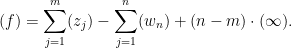
Theorem 40 (Riemann-Hurwitz formula) Let be a non-constant holomorphic map between compact Riemann surfaces of degree , and let be the branch points of this map. Then we have

Furthermore, for any meromorphic -form on , we have

Proof: We begin with the first claim. The space is a -fold cover of . Any triangulation of the latter can then be pulled back to a triangulation of the former with times as many vertices, edges, and faces. As a consequence we have

On the other hand, every time one removes a point from a surface, the Euler characteristic drops by one (we remove one vertex without deleting any edges or faces). Thus

and

Combining these identities with (8), we obtain the first claim.
Next, if we sum (9) over all in the preimage of using (8) we have

and then if one sums over all , one obtain the second claim.
Now we can prove that every canonical divisor on a compact Riemann surface has degree , which is equal to . From Example 23 we see that this claim is true for the Riemann sphere . For any other surface , we use Exercise 37 to produce a non-constant holomorphic map from to the Riemann sphere, and let be any meromorphic -form on the Riemann sphere (e.g. one could take ). Then , hence by both equations in the Riemann-Hurwitz formula we have , and so the canonical divisor has degree . Since all canonical divisors are equivalent, the claim follows.

Exercise 41 Let and be compact Riemann surfaces, with having higher genus than . Show that there does not exist any non-constant holomorphic map from to .

Now we discuss the third claim. It is relatively easy to show that the dimension of the space of holomorphic -forms is upper bounded by . Indeed, we may assume without loss of generality that there exists at least one non-zero holomorphic -form, giving an effective canonical divisor , which we have just shown to have degree . From Proposition 32 applied to we then have

and hence , giving the claimed upper bound.
The lower bound is harder. Basically, it asserts that the pairing in Proposition 32, when quotiented down to a pairing between and , is non-degenerate. This is a special case of an algebraic geometry fact known as Serre duality, which we will not prove here. It can also be proven from Hodge theory, using the fact that the first de Rham cohomology has dimension ; we do not pursue this approach here, but see for instance Griffiths-Harris. Alternatively, one can try to explicitly construct linearly holomorphic -forms on the Riemann surface . We will not do this in general, but show how to do this in the case of a smooth algebraic curve of degree . The genus of such a curve turns out to be given by the genus-degree formula

One can sketch a proof of this using the Riemann-Hurwitz formula. For simplicity of notation let us assume that the polynomial is in “general position” in a number of senses that we will not specify precisely. We can form a holomorphic map

by mapping to . Generically, this will be a non-constant map of degree . The critical points will be those points such that vanishes. As is irreducible of degree , and is irreducible of degree , then Bezout’s theorem will tell us that (generically) there will be critical points , each of multiplicity one (so at each such point ). Applying the Riemann-Hurwitz formula, one concludes that

since and , this gives the genus-degree formula.
To construct linearly independent holomorphic -forms on one can argue as follows. The cases follow from Exercise 8, can be worked out by hand, so suppose . On the projective line , the meromorphic function has a simple pole at , while its differential has a double pole at (and no zeroes). Pulling back by , we see that the meromorphic -form on has double poles at each of the preimages of (making the genericity hypothesis they are distinct and non-degenerate), and also acquire a simple zero at each of the zeroes of . This implies that for any polynomial of degree at most , the -form

is well-defined and holomorphic on the projective curve ) (we have killed all the poles and removed the simple zeroes, while possibly creating new zeroes where vanishes). The space of such polynomials has dimension , giving the claim.
It remains to remove the condition that and be effective to obtain the Riemann-Roch theorem in full generality. We first prove a weaker version known as Riemann’s inequality:

Proposition 42 (Riemann’s inequality) Let be a compact Riemann surface of genus , and let be a divisor. Then .

Proof: Let be a canonical divisor. Choose a non-zero effective divisor such that . We will show that

since from Lemma 19 we have , and , Riemann’s inequality will follow after a brief calculation.
Dividing through by a meromorphic -form of divisor , we see that is the dimension of the space of meromorphic -forms with divisor at least . If with , is the space of meromorphic -forms that have poles of order at most at each , and no other poles.
As in the proof of Proposition 32, let be the space of tuples with complex; this has dimension , and there is a linear map that takes a meromorphic -form in to the tuple of its principal parts at points in . The image is constrained by Proposition 24(i), which forces the residues to sum to zero. On the other hand, by taking linear combinations of the meromorphic -forms from Exercise 37 and Propsosition 38, we see conversely that any tuple in whose residues sum to zero lies in the image of . Thus the image of has dimension . On the other hand, the kernel of is simply the space of holomorphic -forms, which has dimension . The claim follows.
Now we prove the Riemann-Roch theorem. We split into cases, depending on the dimensions of and .
First suppose that and are both positive dimensional. By Exercise 18, is linearly equivalent to an effective divisor, hence by Proposition 32 we have

and similarly (replacing by

and the claim then follows by using .
Now suppose that and are both trivial. Riemann’s inequality then gives

which (again using ) gives , and the claim again follows.
Now suppose that is trivial but is positive dimensional. From Exercise 18 and Proposition 32 as before we have

while from Riemann’s inequality and the triviality of we have

giving the claim. The final case when is trivial and is positive dimensional then follows by swapping with .

Exercise 43 Let be a compact Riemann surface of genus one, and let be a point on . Show that for any points on , there is a unique point on such that is a principal divisor. Furthermore show that this defines an abelian group law on . What is this group law in the case that is an elliptic curve?

Exercise 44 Let be a compact Riemann surface, and suppose that there exists a meromorphic function on with one simple pole and no other poles. Show that is an isomorphism between and the Riemann sphere. Conclude in particular that the Riemann sphere is the only genus zero compact Riemann surface (up to isomorphism, of course).

Exercise 45 Let be a compact Riemann surface of genus , and let be a divisor of degree . Show that when is a canonical divisor, and otherwise.

Exercise 46 (Gap theorems) Let be a compact Riemann surface of genus .

• (i) (Weierstrass gap theorem) If is a point in , show that there are precisely positive integers with the property that there does not exist a meromorphic function on with a pole of order at , and no other poles. Show in addition that all of these integers are less than or equal to .
• (ii) (Noether gap theorem) If are a sequence of distinct points in , show that there are precisely positive integers with the property that there does not exist a meromorphic function with a simple pole at , at most a simple pole at , and no other poles. Show in addition that all of these integers are less than or equal to .

— 5. Appendix: connectedness of irreducible algebraic curves —

In this section we prove

Theorem 47 Let be an irreducible homogeneous polynomial of degree . Then is connected.

We begin with the affine version of this theorem:

Proposition 48 Let be an irreducible polynomial of degree . Then the affine curve

is connected.

We observe that this theorem fails if one replaces the complex numbers by the real ones; for instance, the quadratic polynomial is irreducible, but the hyperbola it defines in is disconnected. Thus we will need properties of the complex numbers that are not true for the reals. We will rely in particular on the fundamental theorem of algebra, the removability of bounded singularities, the generalised Liouville theorem that entire functions of polynomial growth are polynomial, and the fact that the complex numbers remain connected even after removing finitely many points.
We now prove the proposition. We will use the classical approach of thinking of as a branched -fold cover over the complex numbers, possibly after some preparatory change of variables; the main difficulty is then to work around the ramification points of this cover. We turn to the details. Let be an irreducible polynomial of degree , then we can write it as

where for , lies in the space of polynoimals of one variable of degree at most . In particular is a constant. It could happen that this constant vanishes (e.g., consider the example and ); but in that case we will make a change of variables and consider instead the polynomial for a complex parameter . Now the analogue of is a non-trivial polynomial function of (because one of the must have degree exactly ), and so this quantity will be non-zero for some (in fact for all but at most values of ).
Henceforth we assume we have placed into a form where is non-zero. Then, for each , the function is a polynomial of one variable of degree exactly , so it has roots (counting multiplicity) by the fundamental theorem of algebra. Let us call these set of roots , thus

and

From Rouché’s theorem we know that the zero set varies continuously in in the following sense: for any and , each point of will stay within of some point in if is sufficiently close to . (In other words, is continuous with respect to Hausdorff distance.) We also see that the elements in grow at most polynomially in . For some values of , some of these roots in may be repeated. For instance, if , then , which has a double root at if or . However, if this occurs for some , the the degree polynomial and the degree have a common root . This only occurs when the resultant of and vanishes. (One can also use the discriminant of here in place of the resultant; the two are constant multiples of each other.) From the definition of the resultant we see that is a polynomial in , and furthermore we have a Bezout identity

where are polynomials of degree at most and in respectively, with coefficients that are polynomials in . The resultant cannot vanish identically, as this would mean that divides viewed as polynomials in , which contradicts unique factorisation and the irreducibility of since cannot divide the lower degree polynomials or . Thus the resultant can only vanish for a finite number of , and so for all but finitely many the roots of are distinct, thus has cardinality exactly and is non-vanishing at each element of .
From this and the inverse function theorem we see that for outside of a finite number of points (known as ramification points), the set varies holomorphically with . Locally, one can thus describe as a family of holomorphic functions, although the order in which one labels these points is arbitrary, as one varies around one of the ramification points, theis ordering may be permuted (consider for instance the case as goes around the origin, in which we can write for various branches of the square root function).
Now suppose that is disconnected, so it splits into two non-empty clopen subsets . At each non-ramified point , the set meets some subset of . In local coordinates, the are distinct and vary continuously with , the number of points in which meets is locally constant; since with finitely many points removed is connected, this number is then globally constant, thus there is such that has cardinality precisely . This lets us factor , where is the degree polynomial

and is the degree polynomial

The coefficients of these polynomials are functions of that vary holomorphically with outside of the ramification points; they also stay bounded as one approaches these points and grow at most polynomially. Hence (by the generalised Liouville theorem) they depend polynomially on , thus and are in fact a polynomial jointly in . But this contradicts the irreducibility of , unless or . We conclude that is connected after deleting its ramification points. But from the continuous dependence of on , the ramification points adhere to the rest of (the zeroes of are stable under small perturbations, even at points of ramification), so that is connected, proving the proposition.
Now we prove the theorem. The case can be done by hand, so assume . Let be an irreducible homogeneous polynomial of degree . Then is an irreducible polynomial of degree (it cannot be less than , as this will make contain a power of which makes it reducible since ). As a consequence, we see from the proposition that the affine part is connected; similarly if we replace the condition with and . As these three pieces of cover the whole zero locus, it will suffice to show that they intersect each other; for instance, it will suffice to show that the zero set of is not completely contained in any line. But this is clear from the proof of the proposition, which shows that (after a linear transformation) almost every vertical line meets this zero set in points.