Polymath15, tenth thread: numerics update

6 September, 2018 in math.NA, polymath | Tags: Polymath15

This is the tenth “research” thread of the Polymath15 project to upper bound the de Bruijn-Newman constant ${\Lambda}$ , continuing this post. Discussion of the project of a non-research nature can continue for now in the existing proposal thread. Progress will be summarised at this Polymath wiki page.

Most of the progress since the last thread has been on the numerical side, in which the various techniques to numerically establish zero-free regions to the equation $H_t(x+iy)=0$ have been streamlined, made faster, and extended to larger heights than were previously possible. The best bound for $\Lambda$ now depends on the height to which one is willing to assume the Riemann hypothesis. Using the conservative verification up to height (slightly larger than) $3 \times 10^{10}$ , which has been confirmed by independent work of Platt et al. and Gourdon-Demichel, the best bound remains at $\Lambda \leq 0.22$ . Using the verification up to height $2.5 \times 10^{12}$ claimed by Gourdon-Demichel, this improves slightly to $\Lambda \leq 0.19$ , and if one assumes the Riemann hypothesis up to height $5 \times 10^{19}$ the bound improves to $\Lambda \leq 0.11$ , contingent on a numerical computation that is still underway. (See the table below the fold for more data of this form.) This is broadly consistent with the expectation that the bound on $\Lambda$ should be inversely proportional to the logarithm of the height at which the Riemann hypothesis is verified.

As progress seems to have stabilised, it may be time to transition to the writing phase of the Polymath15 project. (There are still some interesting research questions to pursue, such as numerically investigating the zeroes of $H_t$ for negative values of $t$ , but the writeup does not necessarily have to contain every single direction pursued in the project. If enough additional interesting findings are unearthed then one could always consider writing a second paper, for instance.

Below the fold is the detailed progress report on the numerics by Rudolph Dwars and Kalpesh Muchhal.

— Quick recap —

The effectively bounded and normalised, Riemann-Siegel type asymptotic approximation for $H_t(x+yi)$ :

$\displaystyle \frac{H_t(x+yi)}{B_0(x+yi)} = ABB_{eff}(x + iy)+ \mathcal{O}_{\le}(e_A+e_B + e_{C,0})$

enables us to explore its complex zeros and to establish zero-free regions. By choosing a promising combination $y_0$ and $t_0$ , and then numerically and analytically showing that the right-hand side doesn’t vanish in the rectangular shaped “canopy” $x=0 \dots \infty, t = t_0, y=y_0 \dots 1$ (or a point on the blue hyperbola), a new DBN upper bound $\Lambda$ will be established. Summarized in this visual:

numerics1

— The Barrier approach —

To verify that $ABB_{eff} \ne 0$ in such a rectangular strip, we have adopted the so-called Barrier-approach that comprises of three stages (illustrated in a picture below):

numerics2

Use the numerical verification work of the RH already done by others. Independent teams have now verified the RH up to $X=6 \times 10^{10}$ , and a single study took it up to $X=5 \times 10^{12}$ . This work allows us to rule out, up to a certain $X$ , that a complex zero has flown through the critical strip into any defined canopy. To also cover the x-domains that lie beyond these known verifications, we have to assume the RH up to $X$ . This will then yield a $\Lambda$ that is conditional on this assumption.
Complex zeros could also have horizontally flown into the ‘forbidden tunnel’ at high velocity. To numerically verify this hasn’t occurred, a Barrier needs to be introduced at $X$ and checked for any zeros having flown around, through or over it.
Verifying the range $X \leq x < \infty$ (or $N_a \leq N < \infty$ ) is done through testing that the lower bound of $ABB_{eff}$ always stays higher than the upper bound of the error terms. This has to be done numerically up to a certain point $N=N_b$ , after which analytical proof takes over.

So, new numerical computations are required to verify that both the Barrier at $X$ and the non-analytical part of the range $N_a \leq N \leq N_b$ are zero-free for a certain choice of $t_0, y_0$ .

— Verifying the Barrier is zero-free —

So, how to numerically verify that the Barrier is zero-free?

The Barrier is required to have two nearby screens at $X$ and $X+1$ to ensure that no complex zeros could fly around it. Hence, it has the 3D structure: $X \dots X+1, y_0 \dots 1, 0 \dots t_0$ .
For the numerical verification that the Barrier is zero-free, it is treated as a ‘pile’ of $x, y$ rectangles. For each rectangle the winding number is computed using the argument principle and Rouché’s theorem.
For each rectangle, the number of mesh points required is decided using the $\left|\frac{\partial f}{\partial z}\right|$ -derivative, and the t-step is decided using the $\left|\frac{\partial f}{\partial t}\right|$ -derivative.

numerics3

Optimizations used for the barrier computations

To efficiently calculate all required mesh points of $ABB_{eff}$ on the rectangle sides, we used a pre-calculated stored sum matrix that is Taylor expanded in the $x, y$ and $t$ -directions. The resulting polynomial is used to calculate the required mesh points. The formula for the stored sum matrix:

$\displaystyle \mathrm{mat}(I \times J) = {\frac {1}{i!\,j!\,{4}^{j}}\sum _{h=1}^{N}{h}^{i/2x-1/2} \left( \ln \left( 2\,{\frac {h}{N}} \right) \right) ^{i+2\,j}}$

with $i=0 \dots I$ and $j=0 \dots J$ , where $I$ and $J$ are the number of Taylor expansion terms required to achieve the required level of accuracy (in our computations we used 20 digits and an algorithm to automatically determine $I$ and $J$ ).

We found that a more careful placement of the Barrier at an $X+\epsilon$ makes a significant difference in the computation time required. A good location is where $ABB_{eff}$ has a large relative magnitude. Since $ABB_{eff}$ retains some Euler product structure, such locations can be quickly guessed by evaluating a certain euler product upto a small number of primes, for multiple X candidates in an X range.
Since $\left|\frac{\partial f}{\partial z}\right|$ and $\left|\frac{\partial f}{\partial t}\right|$ have smooth i.e. non-oscillatory behavior, using conservative numeric integrals with the Lemma 9.3 summands, $\textrm{summand}_{n=1} + \int_{1}^{N} \textrm{summand dn}$ , instead of the actual summation is feasible, and is significantly faster (the time complexity of estimation becomes independent of $N$ )
Using a fixed mesh for a rectangle contour (can change from rectangle to rectangle) allows for vectorized computations and is significantly faster than using an adaptive mesh. To determine the number of mesh points, it is assumed that $\min ABB_{eff}^{mesh}$ will stay above 1 (which is expected given the way the X location has been chosen, and is later verified after $ABB_{eff}$ has been computed at all the mesh points). The number is chosen as $\bigg \lceil \left|\frac{\partial f}{\partial z}\right| \bigg\rceil$
Since $\min(ABB_{eff}^{mesh})$ for the above fixed mesh generally comes way above 1, the $ABB_{eff}$ lower bound along the entire contour (not just on the mesh points) is higher than what would be the case with an adaptive mesh. This property is used to obtain a larger t-step while moving in the t-direction

$\displaystyle t_{next} = t_{curr} + \frac{\min ABB_{eff}^{mesh} - 0.5}{\big \lceil \left|\frac{\partial f}{\partial t}\right| \big\rceil}$

— Verifying the range $N_a \leq N \leq N_b$ —

This leaves us with ensuring the range $N_a \leq N \leq N_b$ (where $N_a$ is the value of $N$ corresponding to the barrier $X$ ) is zero-free through checking that for each $N$ , the $ABB_{eff}$ lower bound always exceeds the upper bound of the error terms.

From theory, two lower bounds are available: the Lemma-bound (eq. 80 in the writeup) and an approximate Triangle bound (eq. 79 in the writeup). Both bounds can be ‘mollified’ by choosing an increasing number of primes (to a certain extent) until the bound is sufficiently positive.
The Lemma bound is used to find the number of ‘mollifiers’ required to make the bound positive at $N_a$ . We found that using primes $2,3,5,7$ was the max. number of primes still allowing an acceptable computational performance.
The approximate Triangle bound evaluates faster and is used to establish the mollified (either 0 primes or only prime 2) $N_b$ end point before the analytical lower bound takes over.
The Lemma-bound is then also used to calculate that for each $N$ in $[N_a, N_b]$ , the lower bound stays sufficiently above the error terms. The Lemma bound only needs to be verified for the line segment $y=y_0, t=t_0, N_a \leq N(x) \leq N_b$ _, since the Lemma bound monotonically increases when $y$ goes to 1.

numerics4

Optimizations used for Lemmabound calculations

To speed up computations a fast “sawtooth” mechanism has been developed. This only calculates the minimally required incremental Lemma bound terms and only induces a full calculation when the incremental bound goes below a defined threshold (that is sufficiently above the error bounds).

$\displaystyle |f_{N_{min}}| \geq \frac{1}{\sum_{d=1}^D \frac{|\lambda_d|}{d^{\sigma_{N_{min}}}}} \left(1 - |\gamma_{N_{min}}| - \sum\limits_{n=2}^{DN_{min}} \frac{g(n,N_{min},N_{max})}{n^{\sigma_{N_{min}}}} \right)$

$\displaystyle - |\gamma_{N_{min}}| \sum_{n=1}^{N_{min}} \frac{b_n^t (n^{|\kappa|} - 1)}{n^{\sigma_{N_{min}}-y}}$

$\displaystyle|f_{N+1}| := |f_{N}| - \frac{1}{\sum_{d=1}^D \frac{|\lambda_d|}{d^{\sigma_{N+1}}}} \sum\limits_{1 \leq d \leq D:d|D}(\sum\limits_{n=dN+1}^{dN+d} \frac{g(n,N_{min},N_{max})}{n^{\sigma_{N+1}}}) - |\gamma_{N+1}| \frac{b_{N+1}^t ({(N+1)}^{|\kappa|} - 1)}{(N+1)^{\sigma_{N+1}-y}}$

where

$\displaystyle g(n,N,N_{max}) = \max(\frac{1-|\gamma|_{N_{max}}}{1+|\gamma|_{N_{max}}} |\beta_{n,N} + \alpha_{n,N}|,$

$\displaystyle|\beta_{n,N} - \alpha_{n,N}|, |\beta_{n,N} - |\frac{\gamma_{N_{max}}}{\gamma_{N}}| \alpha_{n,N}|)$

(as presented within section 9 of the writeup, pg. 42)

— Software used —

To accommodate the above, he following software has been developed in both pari/gp (https://pari.math.u-bordeaux.fr) and ARB (http://arblib.org):

For verifying the Barrier:

Barrier_Location_Optimizer to find the optimal $X, X+1$ location to place the Barrier.
Stored_Sums_Generator to generate in matrix form, the coefficients of the Taylor polynomial. This is one-off activity for a given $X$ , post which the coefficients can be used for winding number computations in different $y$ and $t$ ranges.
Winding_Number_Calculator to verify that no complex zeros passed the Barrier.

For verifying the $N_a \leq N \leq N_b$ range:

N_b_Location_Finder for the number of mollifiers to make the bound positive.
Lemmabound_calculator Firstly, different mollifiers are tried to see which one gives a sufficiently positive bound at $N_a$ . Then the calculator can be used with that mollifier to evaluate the bound for each $N$ in $[N_a,N_b]$ . The $[N_a,N_b]$ range can also be broken up into sub-ranges, which can then be tackled with different mollifiers.
LemmaBound_Sawtooth_calculator to verify each incrementally calculated Lemma bound stays above the error bounds. Generally this script and the Lemmabound calculator script are substitutes for each other, although the latter may also be used for some initial portion of the N range.

Furthermore we have developed software to compute:

$ABB_{eff}$ as $\left|\frac{A+B}{B_0}\right|$ and/or $\left|\frac{A+B-C}{B_0}\right|$ .
the exact $H_t(x+iy)$ value (using the bounded version of the 3^rd integral approach).

The software supports parallel processing through multi-threading and grid computing.

— Results achieved —

For various combinations of $y_0, t_0$ , these are the numerical outcomes:

numerics5

The numbers suggest that we now have numerically verified that $\Lambda \le 0.22$ (even at two different Barrier locations). Also, conditionally on the RH being verified up to various $x > 6 \times 10^{10}$ , we have now reached a $\Lambda \le 0.12$ . We are cautiously optimistic, that the tools available right now, do even bring a conditional $\Lambda \le 0.10$ within reach of computation.

— Timings for verifying DBN $\le 0.22$ —

Procedure	Timings
Stored sums generation at X=6*10^10 + 83951.5	42 sec
Winding number check in the barrier for t=[0,0.2], y=[0.2,1]	42 sec
Lemma bounds using incremental method for N=[69098, 250000] and a 4-prime mollifier {2,3,5,7}	118 sec
Overall Timings	~200 sec

Remarks:

Timings to be multiplied by a factor of ~3.2 for each incremental order of magnitude of x.
Parallel processing significantly improves speed (e.g. Stored sums was done in < 7 sec).
Mollifier 2 analytical bound at $N=250,000, y=0.2, t=0.2$ is $~ 0.098$ .

— Links to computational results and software used: —

Numerical results achieved:

Stored sums https://github.com/km-git-acc/dbn_upper_bound/tree/master/output/storedsums
Winding numbers https://github.com/km-git-acc/dbn_upper_bound/tree/master/output/windingnumbers

Lemmabound N_a…N_b https://github.com/km-git-acc/dbn_upper_bound/tree/master/output/eulerbounds

Software scripts used:

ARB-software https://github.com/km-git-acc/dbn_upper_bound/tree/master/dbn_upper_bound/arb
pari/gp-software https://github.com/km-git-acc/dbn_upper_bound/tree/master/dbn_upper_bound/pari

104 comments

Comments feed for this article

6 September, 2018 at 11:06 pm

scienaimer

Thanks😄, I admire you so much

13 October, 2018 at 11:22 am

Anonymous

Please don’t forget to take that ceremonial bow when you think his or speak his name… :-)

P.S. And trust me, he is a bit overrated too.

18 October, 2018 at 7:31 am

Anonymous

On the other hand, Prof. T. Tao has established a first-rate and evolving website on mathematics (https://terrytao.wordpress.com), and it may be the best on the worldwide internet. Thank you very much! :-)

7 September, 2018 at 7:12 am

Anonymous

Is it possible to reduce the computational complexity by making the width of the barrier variable (not necessarily 1) and choosing a “good” value for it ?

7 September, 2018 at 7:30 am

Terence Tao

The barrier can be reduced in area by a factor of about two (at the cost of replacing its rectangular shape with a region bounded by two straight lines and a parabola), but it can’t be made arbitrarily small (at least with the current arguments). The reason why the barrier needs to be somewhat thick is because one needs to ensure that the complex zeroes (paired with their complex conjugates) on the right of the barrier cannot exert an upward force on any complex zero above the real axis to the left of the barrier; this is to prevent the bad scenario of a complex zero swooping in under the barrier at high velocity, and then being pulled up by zeroes still to the right of the barrier to end up having an imaginary part above $y_0$ at the test time $t_0$ . If the barrier is too thin, then a zero just to the left of it could be pulled up strongly by a zero just to the right and a little bit higher, to an extent that cannot be counteracted by the complex conjugate of the zero to the right. (Though, as I write this, I realise that also the complex conjugate of the zero on the left would also be helpful in pulling the zero down. This may possibly help reduce the size of the barrier a little bit further, although it still can’t be made arbitrarily thin. I’ll try to make a back-of-the-envelope calculation on this shortly. EDIT: ah, I remember the problem now… if one has _many_ zeroes on the right of the barrier trying to pull the zero on the left up, they can overwhelm the effect of the complex conjugate of that zero, so one can’t exploit that conjugate unless one also has some quantitative control on how many zeroes there are just to the right of the barrier.)

My understanding is that verification that the barrier is zero-free has not been the major bottleneck in computations, with the numerical verification of a large rectangular zero-free region to the right of the barrier at time $t_0$ being the more difficult challenge, but perhaps the situation is different at very large heights (I see for instance that there is one choice of parameters in which the rectangular region is in fact completely absent).

7 September, 2018 at 12:19 pm

If we use the Euler 2 analytic bound, and try to maintain the trend of the dbn constant decreasing by 0.01 or more for every order of magnitude change in X, without having to validate any rightward rectangular region, we find such good t0,y0 combinations only till X=10^19.

For example, for X=10^20, we don’t find a combination which could give dbn <= 0.11 by itself (although 0.1125 is manageable), and validating an extra region becomes necessary. We could instead assume a new such trend starts at X=10^20 and ends at X=10^22 with dbn going from 0.12 to 0.10.

If we validate a rightward rectangular region at these heights, it does take significant time. Here, the stored sums generation also takes substantial time (for eg. the 10^19 stored sums took about 30 processor-days (although quite parallelized)). We can choose a larger X to eliminate or reduce the rectangular region but at the cost of more time for the stored sums.

7 September, 2018 at 11:45 am

curious

With unbounded computation capability and infinite time is there a lower bound on $\Lambda$ ?

7 September, 2018 at 4:24 pm

Terence Tao

Well, it’s now a theorem that $\Lambda \geq 0$ , and the Riemann hypothesis is now known to be equivalent to $\Lambda=0$ , so it is unlikely that this lower bound will ever be improved :)

Conversely, in the unlikely event that we were able to numerically locate a violation of the Riemann hypothesis, that is to say a zero of $H_0$ off the real line, one could hopefully use some of the numerical methods to calculate $H_t$ developed here to also locate failure of the Riemann hypothesis at or near this location for some positive values of $t$ as well. This would then give a positive lower bound to $\Lambda$ . But I doubt this scenario will ever come to pass. (I doubt that RH will ever be disproven, but if it is, my guess is that the disproof will come more from analytic considerations than from numerically locating a counterexample, which might be of an incredibly large size (e.g., comparable to Skewes number).)

16 October, 2018 at 8:56 am

Anonymous

Your arguments/doubts against the truth of the Riemann Hypothesis are fictional, and therefore, they should be ignored…

7 September, 2018 at 1:15 pm

Anonymous

In step 4 (of “verifying the range”), the meaning of “the line $y_0, t_0$ ” is not clear.

[Text clarified – T.]

7 September, 2018 at 5:31 pm

Anonymous

It seems that $y = t_0$ should be $t = t_0$ .

[Corrected, thanks – T.]

7 September, 2018 at 1:21 pm

Anonymous

It is possible to prove that $\Lambda \geq 0$ using the zero-free regions method? For example, prove that $\Lambda \geq \varepsilon$ for every positive $\varepsilon$ ?

7 September, 2018 at 4:26 pm

Anonymous

What you are asking for is a proof that the Riemann hypothesis fails.
RH implies lambda <= 0.

7 September, 2018 at 4:34 pm

Anonymous

Sorry… i wanted to say $\Lambda \leq 0$ . I wasn’t pay atention. Thanks!

7 September, 2018 at 4:49 pm

Terence Tao

As I think I mentioned in the previous thread, establishing an upper bound $\Lambda \leq \varepsilon$ is roughly comparable in difficulty to verifying the Riemann hypothesis up to height $\exp(C/\varepsilon)$ for some absolute constant $C$ . The computational difficulty of this task is in turn of the order of $\exp(C'/\varepsilon)$ for some other absolute constant $C'$ . So the method can in principle obtain any upper bound of the form $\Lambda \leq \varepsilon$ (assuming of course that RH is true), but the time complexity grows exponentially with the reciprocal of the desired upper bound $\varepsilon$ . My feeling is that absent any major breakthrough on RH, these exponential type bounds are here to stay, although one may be able to improve the values of $C$ and $C'$ somewhat.

16 October, 2018 at 9:03 am

Anonymous

“… major breakthrough on RH…” Hah! RH is true!… And your acceptance of this fact will be your personal breakthrough!

7 September, 2018 at 6:55 pm

curious

Does the $\exp(C/\epsilon)$ behavior come from proposition 10.1? Also you say it is unlikely to beat $\log T\Lambda=O(1)$ and perhaps it would be nice to state the best behavior if it is beaten to $\log T\Lambda=o(1)$ and what is the unlikely event that would trigger?

7 September, 2018 at 7:42 pm

Terence Tao

See my previous comment on this at https://terrytao.wordpress.com/2018/05/04/polymath15-ninth-thread-going-below-0-22/#comment-501625

21 September, 2018 at 5:55 am

Anonymous

Stay tuned:
https://www.newscientist.com/article/2180406-famed-mathematician-claims-proof-of-160-year-old-riemann-hypothesis/

21 September, 2018 at 7:02 am

Anonymous

Such claim from him seems really promising …

22 September, 2018 at 9:26 pm

Anonymous

Dear Prof. Tao,

Are you aware of any details on the supposed proof of the RH by Atiyah?

Best,

23 September, 2018 at 12:22 pm

sylvainjulien

There’s a question on Mathoverflow with a link towards a preprint by Sir Michael : https://mathoverflow.net/questions/311254/is-there-an-error-in-the-pre-print-published-by-atiyah-with-his-proof-of-the-rie

24 September, 2018 at 6:32 am

sha_bi_a_ti_ya

hi, the link does not work any more.

24 September, 2018 at 6:02 am

Anonymous

The papers are out and basically it seems that there is a consensus among the experts that the proof is incorrect (e.g. https://motls.blogspot.com/2018/09/nice-try-but-i-am-now-99-confident-that.html).

I would really like to read a comment on this from prof. Tao.

24 September, 2018 at 6:58 am

think

Motls is no expert.

24 September, 2018 at 8:53 am

Anonymous

Dear prof. Tao,

I suggest to delete this discussion on the claimed proof as irrelevant to this post.

24 September, 2018 at 9:22 am

Anonymous

How is a possible proof of RH not relevant to a bound on the roots of zeta function? Once there is a proof of RH being true, \Lambda = 0 and there is no need for the numerics.

9 October, 2018 at 12:26 am

Anonymous

Interestingly, for some comments above, the “authomatic dislike” is missing.

24 September, 2018 at 9:52 am

Terence Tao

Given the situation, I believe it would not be particularly constructive or appropriate for me to comment directly on this recent announcement of Atiyah. However, regarding the more general question of evaluating proposed attacks on RH (or GRH), I can refer readers to the recent talk of Peter Sarnak (slides available here) entitled “Commentary and comparisons of some approaches to GRH”. A sample quote: “99% of the ‘proofs’ of RH that are submitted to the Annals … can be rejected on the basis that they only use the functional equation [amongst the known properties of $\zeta$ , excluding basic properties such as analytic continuation and growth bounds]”. The reason for this is (as has been known since the work of Davenport and Heilbronn) that there are many examples of zeta-like functions (e.g., linear combinations of L-functions) which enjoy a functional equation and similar analyticity and growth properties to zeta, but which have zeroes off of the critical line. Thus, any proof of RH must somehow use a property of zeta which has no usable analogue for the Davenport-Heilbronn examples (or the many subsequent counterexamples produced after their work, see e.g., this recent paper of Vaughan for a more up-to-date discussion). (For instance, the proof might use in an essential way the Euler product formula for zeta, as the Davenport-Heilbronn examples do not enjoy such a product formula.)

Another “barrier” to proofs of RH that was mentioned in Sarnak’s talk is also worth stating explicitly here. Many analysis-based attacks on RH would, if they were successful, not only establish that all the non-trivial zeroes lie on the critical line, but would also force them to be simple. This is because analytic methods tend to be robust with respect to perturbations, and one can infinitesimally perturb a meromorphic function with a repeated zero on the critical line to have zeroes off the critical line (cf. the “dynamics of zeroes” discussions in this Polymath15 project). However, while the zeroes of zeta are believed to be simple, there are many examples of L-functions with a repeated zero at 1/2 (particularly if one believes in BSD and related conjectures). So any proof of RH must either fail to generalise to L-functions, or be non-robust with respect to infinitesimal perturbations of the zeta function. (For instance, in Deligne’s proof of the RH for function fields, the main way this barrier is evaded is through the use of the tensor power trick, which is not robust with respect to infinitesimal perturbations. This proof also evades the first barrier by relying in essential fashion on the Grothendieck-Lefschetz trace formula, which is not available in usable form for Davenport-Heilbronn type examples, even over function fields.)

(I also spoke at this meeting, on the topic of the de Bruijn-Newman constant and (in part) on Polymath15; my talk can be found here, and the remaining lectures may be found here, with slides here.)

24 September, 2018 at 10:40 am

Anonymous

On the other hand, Hamburger’s theorem (1921) shows that $\zeta$ is determined (up to a multiplicative constant) by its functional equation, having Dirichlet series representation, finitely many singularities and growth conditions. So in addition to the functional equation and Dirichlet series representation not much more information is needed for a proof of RH.

24 September, 2018 at 12:55 pm

Terence Tao

This is true insofar as one restricts attention just to RH rather than GRH. But at the GRH level one needs the functional equation not just for the Dirichlet series, but for all twists of the Dirichlet series, in order to recover an L-function (or at least to evade the Davenport-Heilbronn type counterexamples). So any purported proof of RH that relies only on the functional equation and the Dirichlet series representation must either fundamentally break down when one attempts to extend it to GRH (i.e., it must use some special property of zeta not shared by other L-functions, such as the specific numeric parameters that appear in the gamma factors of the zeta functional equation as opposed to all other functional equations, which by the way is the case for Hamburger’s theorem), or must naturally incorporate the functional equation for the twists as well. (One could possibly imagine the latter occurring if the argument had a highly “adelic” flavour, for instance.)

25 September, 2018 at 11:13 am

Aula

Since Deligne managed to prove one special case of GRH, it’s a pretty obvious idea to try to generalize his proof to other cases. However it seems that no one has been able to do so, which suggests that function fields really are a very special case of GRH. Why is that?

25 September, 2018 at 12:03 pm

Terence Tao

Well, the function field case is more like half of all cases (if one considers the function field case and number field case to be of equal “size”); Deligne proved GRH not only for the analogue of the zeta function and Dirichlet L-functions (which are actually quite easy), or for curves (which was first done by Weil), but in fact proved GRH for all varieties and more generally for “pure” l-adic sheaves. (See my previous blog post on this at https://terrytao.wordpress.com/2013/07/19/the-riemann-hypothesis-in-various-settings/ .)

Probably the most obvious thing that the function field case has but the number field case seems to lack is the Frobenius map, which is linked to L-functions in the function field case via the Grothendieck-Lefschetz trace formula. But people have certainly searched for ways to extend these methods to number field settings, most prominently Connes and his co-authors (see e.g., his recent talk (slides available here), at the same conference as the previously linked talks). Connes identifies the apparent lack of a (Hirzebruch-)Riemann-Roch theorem for number fields as the key obstacle to making this strategy work.

22 October, 2018 at 3:50 pm

Anonymous

Since RH is generally regarded as the most important open conjecture in mathematics (with many claimed proofs), it seems that any accepted proof of it should also be formalized.

26 October, 2018 at 1:41 pm

Anonymous

Some recently claimed proofs of RH (with some remarks)
http://www.maths.ex.ac.uk/~mwatkins/zeta/RHproofs.htm

7 June, 2022 at 9:13 am

kirill kapitonets

Dear prof. Tao,

Let me make a few comments about the aspects of Peter Sarnak’s speech that you have cited.

The Davenport and Heilbronn functions differ significantly from the Riemann Zeta functions, although one and the other correspond to the functional equation. This difference lies in the concept of linear dependence, i.e. the ability to express the values of a function on one line parallel to the critical line and some other line also parallel to the critical line, i.e. with different values of the real part of the complex variable. For the Davenport and Heilbronn functions, such a linear dependence is true for any two values of a real variable, which does not contradict the functional equation, while for the Riemann Zeta function, such a linear dependence is established by the functional equation only for lines symmetric with respect to the critical line, therefore, on all other lines parallel to the critical line, the values of the Riemann Zeta function are linearly independent. This linear independence leads to a special property of the Riemann Zeta function – the values of the Riemann Zeta function on rational lines parallel to the critical line, i.e. taken at different rational values of the real part of a complex variable, form the basis of a Hilbert space, and the Davenport and Heilbronn function does not have this property. Therefore, in this case, it is not the functional equation that is important, but the linear independence, which is described above.

Now as for the second remark about simple zeros. Some considerations suggest that it is necessary to move from a function of a complex variable to a function of a real variable. To do this, it is enough to take the real part of the Riemann Zeta function, domnazhaya it by a known multiplier, which is used to obtain the function of a real variable on the critical line to calculate the zeros of the Riemann zeta function. This function is sometimes called the Hardy function. Then using the properties of the Riemann Zeta function to have linearly independent values on lines parallel to the critical line, we obtain a generalized Hardy function that also has linearly independent values on lines parallel to the critical line. Consequently, the generalized Hardy function on rational lines parallel to the critical line, i.e. taken at different rational values of the real part of a complex variable, form the basis of a Hilbert space over the field of real numbers. Further, some considerations allow us to assert that the functions that make up the basis of a Hilbert space over a field of real numbers have all simple real zeros (they inherit this property from real orthogonal polynomials, which are elements of the best approximation in a Hilbert space). Thus, the property of linear independence of the values of the Riemann Zeta function on lines parallel to the critical line and not satisfying the functional equation is responsible for the property of zeros of the Riemann Zeta function – they are all simple and of course all lie on the critical line, because The Hardy function belongs to the Hilbert space basis.

Let me ask you what you think about this?

Maybe it’s a double, because I don’t see the first message.

25 September, 2018 at 12:53 am

think

Is it possible RH is true but not GRH and may be is there possibility in that case your reasoning might fall short?

25 September, 2018 at 6:47 am

Terence Tao

This is theoretically possible, but (a) it goes against the experience of the last century or so, in which virtually every property that has been established for the zeta function eventually ends up having an analogue for other L-functions (possibly with some additional subtleties), and (b) as I said above, it would mean that any proof of RH would at some point have to rely in some crucial fashion on a property of the zeta function that has no usable analogue for L-functions (i.e., it must use an exception to (a)), since otherwise it would extend to a proof of GRH, which we are assuming for this discussion to be false. Again, this is theoretically possible – certainly I could imagine for instance that there would be an argument that can handle degree 1 L-functions such as zeta or Dirichlet L-functions, but not higher degree L-functions – but many attacks on RH would not be able to make such fine distinctions between zeta and other L-functions, e.g., arguments that are primarily based on complex analysis methods. (The only exception I could see is if the argument really used the specific value of the numerical exponents and other parameters of the zeta functional equation in some key fashion, so that the argument would break down completely if these parameters were replaced by those for some other L-function. Hamburger’s theorem, mentioned above, is one case in which this occurs.)

EDIT: my previous discussion on the distinction between local errors in a proof and global errors in a proof is relevant here. A local error is something like “The derivation of equation (23) on page 17 is not valid” or “The proposed definition of a pseudosimplicial hypercomplex in Definition 3.1 is ambiguous”. A global error is something like “this proof, if it worked, would also show that all meromorphic functions obeying the functional equation must verify the Riemann hypothesis, which is known not to be the case”. A good proof should not only be written in a way to avoid local errors, but also should be consciously striving to avoid global ones as well, otherwise it immediately becomes suspicious (even if the specific local error that the global error indicates must exist has not yet been located).

25 September, 2018 at 9:12 am

think

Not sure if there is a relation but from https://terrytao.wordpress.com/2018/01/19/the-de-bruijn-newman-constant-is-non-negativ/ even RH seems to be barely so. Any non-negativity statement like this holds for GRH?

25 September, 2018 at 10:16 am

Anonymous

It seems that the “barely so” result for the “de-Bruijn” deformation $H_t$ for $H_0$ is “too rigid” for the deformation parameter $t$ , so perhaps the “epsilon of room” principle indicates that it may be useful to make the deformation more flexible by using several deformation parameters ( $t, t_1$ , say) instead of the single parameter t.
This may be used to get some desirable properties of the more general deformation. Such a desirable property is to rigorously bound the zeros velocities of $H_{t, t_1}$ by using instead of the classical heat equation (which has unbounded propagation velocities) by a similar version of “relativistic heat equation” (with a small parameter of second order time derivative corresponding to a “wave equation” which should give the desired upper bound on the propagation velocity).See e.g.
https://en.wikipedia.org/wiki/Relativistic_heat_conduction

25 September, 2018 at 11:56 am

Terence Tao

I am actually planning to ask a graduate student to look into this question.

27 September, 2018 at 4:20 am

Anonymous

Is it possible to refine de Bruijn deformation $H_t$ of $H_0$ to a more general (two parametric) deformation $H_{t, t'}$ such that

(i) $H_{t, t'}$ converges locally uniformly to $H_0$ as $(t, t')$ tend to $(0, 0)$ .

(ii) For each $t, t' > 0$ there is $X(t, t')$ such that 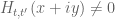$H_{t, t'}(x+i y) \neq 0$ whenever $x > X(t, t')$ and $y > 0$ .

(iii) The threshold $X{t, t'}$ is effectively computable.

Such a generalized deformation may be derived from a relativistic version of the heat equation. It seems that if there is a sequence of deformation parameters $(t_n, t'_n)$ converging to $(0, 0)$ with a corresponding sequence of thresholds $X(t_n, t'_n)$ uniformly bounded by some absolute constant M, then property (i) would imply that 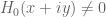$H_0(x + i y) \neq 0$ whenever $x > M$ and $y > 0$ .

2 October, 2018 at 3:57 pm

Anonymous

A similar “deformation approach” to RH is to represent the kernel $\Phi$ (which gives $H_0$ as its Fourier transform) as a limit of a suitable sequence of kernels whose Fourier transforms have only real zeros and are converging locally uniformly to $H_0$ – implying that H_0 has also only real zeros. This “kernel deformation approach” appears in Shi’s recent arxiv paper

Click to access 1706.08868.pdf

3 October, 2018 at 4:42 am

Anonymous

A more detailed description of the “kernel deformation approach” to RH is as follows

Since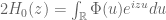 $2 H_0(z) = \int_{\mathbb{R}} \Phi(u) e^{i z u} d u$ , where $H_0$ is entire with its double-exponentially decaying “generating kernel” $\Phi$ , the basic idea is to construct a sequence of “approximating kernels” $\Phi_n$ to $\Phi$ whose Fourier transforms
$F_n(z) := \int_{\mathbb{R}} \Phi_n(u) e^{i z u} d u$ should be

(i) well-defined and analytic in the horizontal strip $|y| < 1$ .
(ii) converging locally uniformly to $2 H_0$ in this strip.
(iii) have only real zeros in this strip.

Clearly, the above properties imply that $H_0$ has only real zeros!

Remarks:

1. A sufficient condition for property (i) is

$\int_{\mathbb{R}} |\Phi_n(u)| e^{|u|} d u < \infty$ for each $n$

2. A sufficient condition for property (ii) is

$\lim_{n \to \infty} \int_{\mathbb{R}} |\Phi_n(u) -\Phi(u)| e^{|u|} d u=0$

which follows from the simple estimate (in the strip $|y| < 1$ )

$|F_n(z) - 2 H_0(z)| \leq \int_{\mathbb{R}} |\Phi_n(u)-\Phi(u)| |e^{i z u}| d u$

$\leq \int_{\mathbb{R}} |\Phi_n(u) - \Phi(u)| e^{|u|} d u$

3. It seems that satisfying property (iii) is the most difficult part in the construction (or "design") of such kernels $\Phi_n$ .

3 October, 2018 at 7:57 am

sha_bi_a_ti_ya

bro, are you mr. shi?

2 October, 2018 at 4:01 pm

Terence Tao

I am not sure I fully understand your set of hypotheses, but it appears that $H_{t,t'} := H_t$ already obeys the properties you state (but with the threshold not bounded uniformly in $t,t'$ ).

2 October, 2018 at 4:21 pm

Anonymous

Yes, it is true for the one-parameter deformation $H_t$ , but perhaps the extra flexibility of the two-parametric deformation $H_{t, t'}$ may be sufficient to have a suitable sequence of such deformations converging locally uniformly to $H_0$ while keeping their corresponding thresholds uniformly bounded?
Moreover, if the deformation $H_{t, t'}$ is generated from a relativistic version of the heat equation (with bounded propagation velocity), is it possible that their zeros velocities are also uniformly bounded?

28 September, 2018 at 12:33 pm

vznvzn

led from an offhand remark/ tip by a commenter on RJLs recent blog on atiyah attack, now delighted/ excited/ exhilarated to see this hard core empirical/ computational/ numerical work into RH and hope that the word gets out, there are apparently multiple trolls on my blog who reject my own similar inquiries into collatz on spurious grounds. does anyone know of a great survey ref on RH numerical work or more widely in number theories? have found a few of my own over the years but have to go hunt down some of these new refs. https://vzn1.wordpress.com/2015/12/29/select-refs-and-big-tribute-to-empirical-cs-math/

re Atiyah attack, spent a lot of time researching that from many angles, this is a pov written from an outsider looking in on all the insiders. https://vzn1.wordpress.com/2018/09/26/atiyah-riemann-attack-post-mortem-autopsy-primes-torch-carried-on/

29 September, 2018 at 2:56 pm

Terence Tao vs Riemann Hypothesis, polymath 15 computational/ algorithmic number crunching attack, counterpoint to recent Atiyah episode - Nevin Manimala's Blog

[…] by /u/vznvzn [link] […]

29 September, 2018 at 5:39 pm

Atiyah Riemann attack/ post mortem/ autopsy, Primes torch carried on | Turing Machine

[…] thx everyone! from a comment on RJLs blog about "number crunching Riemann", Terence Tao/ Polymath15 is working on a very cool numerical attack. more vindication for numerical approaches. reddit likes […]

1 October, 2018 at 4:29 am

Anonymous

More information on Todd function (appearing in Atiyah claimed proof for RH) and on the closely related Hirzebruch functional equation can be found in Bunkova’s recent arxiv paper

Click to access 1803.01398.pdf

7 October, 2018 at 5:29 pm

Anonymous

In the writeup, it seems that in the RHS of (33) the argument of the logarithmic derivative should be $z$ (instead of $z_j$ ).
In addition, the proof of claim (i) (in the following rows) can be simplified by observing that the Hadamard product for $H_t$ is locally uniformly convergent – implying that its logarithmic derivative is also locally uniformly convergent – so the logarithmic derivative can be computed termwise and the claim follows (without relying on growth estimates.)

[Thanks, the LaTeX source has now been updated (and the PDF will be updated in due course). -T]

8 October, 2018 at 11:41 am

Anonymous

Since $H_0$ can be represented as the Fourier transform of a (fast decaying) strictly positive definite function $\Phi$ , it is therefore a positive definite function on $\mathbb {R}$ (such positive definite functions are characterised by Bochner’s theorem as Fourier transforms of positive functions.)
Is it possible that $H_0$ represents the correlation function of a stationary continuous-time random process on $\mathbb{R}$ with $\Phi$ as its corresponding power spectral density? (which may explain the empirical connection of the distribution of $H_0$ zeros to the distribution of eigenvalues of large random Hermitian matrices.)

10 October, 2018 at 9:55 am

Watching Over the Zeroes | Gödel's Lost Letter and P=NP

[…] results toward the RH. A PolyMath project on bounding from above has achieved , and a bound of is known to follow if and when the RH is verified for up to . There was previously a lower bound , a […]

13 October, 2018 at 10:16 am

Anonymous

Since $\Phi_t(u) := e^{t u^2} \Phi (u)$ is the integral kernel representing $H_t(z)$ , it seems desirable to understand in terms of the kernel $\Phi_t$ why it makes some zeros of $H_t$ non-real for $t 0$ . (i.e. which property of the kernel is changing at the threshold $t = 0$ ?)
It is known from a classical paper (1918) of Polya that if the kernel is even, INCREASING function for $u > 0$ and compactly supported, its Fourier transform (which is a finite cosine transform) is an entire function with only real zeros. If the kernel function is DECREASING (as in the case of $\Phi$ ), its Fourier transform may have non-real zeros (there are some results connecting its convexity properties to the zeros distribution of its Fourier transform). Since the derivative of $\Phi$ (as any even function) is zero at the origin, is it possible that its second derivative at the origin is also zero – which would make $\Phi_t$ CONVEX at the origin $u = 0$ for $t > 0$ , but CONCAVE for $t < 0$ ?
(thereby explaining its convexity "transition" at the origin $u=0$ for $t = 0$ ).

13 October, 2018 at 10:22 am

Anonymous

Correction: in the fourth line it should be “for $t < 0$ " (i.e. "<" is missing)

8 December, 2018 at 5:39 pm

Anonymous

What about Atiyah’s proof of Riemann Hypothesis? There are 100 percent of chance that his demonstration are wrong?

22 December, 2018 at 8:51 am

Anonymous

From reading between the lines on the internet, it sadly looks like his proof is so nonsensical that it cannot be described without implying that he suffers from some sort of neurodegenerative disorder. If you want to avoid the appearance of making a remote amateur diagnosis of his medical condition then you have to talk around it by referring obliquely to “the situation” and by listing known barriers to proofs in general instead of explaining his proof in particular.

9 December, 2018 at 10:22 am

Is there any update on polymath15? In particular, I have seen that the writeup-directory has not been changed for 3 weeks. Is there something that other people, who potentially have not been involved, could contribute on the writing part? For example, some final proof-reading etc? Would be nice to get some updates from the involved researchers.

9 December, 2018 at 2:09 pm

Anonymous

I’m not as involved as the authors of the numerics report, but I’ve been casually involved in the past and I still read the mailing list occasionally. There are three main reasons that I’ve decreased my participation in the project. One is that I wasn’t able to follow the details of “a pre-calculated stored sum matrix that is Taylor expanded” and I don’t know if it’s rigorously proved or if it’s heuristics or what. I assume this is my fault for not understanding. Secondly the project shifted towards looking at negative values of t. I’m not going to tell other people what to work on, but it looked out of scope for this project. Thirdly the active research on this project currently appears to be numerically extending the number of zeros checked on the critical line which I think is way outside this scope of this project. If you can prove a result that has a dependency on how many zeros have been checked then I feel like that’s enough. You don’t have to keep trying to check more zeros, except as a spinoff project. I’m not trying to be negative or discouraging, I think this is a great project and the people working on it are great, I’m just giving an update from my own perspective and explaining why my own participation has declined.

10 December, 2018 at 7:45 am

Terence Tao

The main thing missing from the writeup currently is basically a detailed explanation of the numerics used (in particular the stored sum thing you allude to). Once I have a block of time in which I can verify some of the code I should be able to fill that in, and then one just needs some proofreading and polishing before one can submit the writeup which would I think close off the original goal of Polymath15, though the secondary goals of exploring negative t and seeing if one can expand (or reconfirm) the range of numerical verification of RH are also interesting. The (extraordinarily busy) quarter has just ended for me, so after this AIM workshop that I am at this week concludes, I should be able to finally have that block of time…

18 December, 2018 at 10:14 am

rudolph01

Here is a quick update from the numerics team. Since September we have progressed work along three lines:

1) In our quest to further reduce the DBN-constant below $0.22$ , i.e. the domain where results will be conditional on RH-verification up to a certain height, we found a new approach. The table under ‘results achieved’ in the OP of the 10th thread, has an interesting row (the 3rd from below) where for a carefully chosen combination of $y_0, t_0$ , the Triangle bound $N_b$ is already positive at the location of the Barrier. This implies $N_a=N_b$ , hence no further computations are required after the Barrier has been ‘cleared’ from any zeros having passed through it. This brought us to the idea to find those $x, y_0, t_0$ combinations for which the Triangle bound just becomes (and stays) positive and then to place the Barrier at an optimal location just beyond the derived x-value. This approach, combined with having access to a powerful grid-computing environment (Boinc), allowed us to numerically prove a conditional DBN of $\le 0.10$ . Here is the table with the results achieved.

2) Since these results are conditional on the RH and we had gained access to the powerful grid environment, we decided to explore the previous verification work done on the RH (Brent, Hugh, Riele/Lune, Wedeniwski, Gourdon, Platt, etc.). This to see whether existing algorithms might be replicated in the modern ARB-software (http://arblib.org) and thereby maybe stretch the verified heights a bit further. The current status is that we have produced scripts to count the zeros on the critical line as well as to count those in the strip (via Turing’s method). Using grid computing, this probably brings verification up till the first $10^{11}$ zeros ( $x = 3 \times 10^{10}$ within reach. This is the same height as Platt’s achieved and the one used for our unconditional DBN=0.22 proof. Beyond this level, the ‘factor 10’ increments quickly require much more advanced techniques than the classical Riemann-Siegel formula to evaluate $Z(s)$ . This is where the various Odlyzko-Schönhage algorithms kick in and given their complexity these should clearly be left to the experts in this field. So, we probably will only complete a verification run up till $10^{11}$ and then ‘return’ from this brief out-of-the-project-scope subroutine.

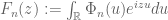
3) Our third work stream focuses on the visualisation of the trajectories of the real and complex zeros in the (larger) negative t-domain. We have struggled for a while to get to a stable function to adequately explore this territory. The only tool currently available that remains valid at larger negative $t$ , is this integral,

$H_t(z) = \frac{1}{8\sqrt{\pi}}\int^{k}_{-k} \xi\left(\frac{1+iz}{2} + \sqrt{t}\, v \right) e^{-v^2} \mathrm{d}v$

and its first derivative:

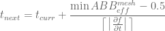
$H_t^{'}(z) = \dfrac{i}{8\sqrt{\pi\,t}}\int_{-k}^{k}\,\xi\left(\frac{1+i\,z}{2}+\sqrt{t} v\right) e^{-v^2} v\,\mathrm{d}v$

These integrals quickly become difficult to evaluate at more negative $t$ . After some experiments we found that approaching the integral by a sum of rectangles with $k$ and the rectangle widths as key parameters. This approach made it more effectively controllable, however negative t smaller than -100 remain a stretch. The $latexH_t$-derivative is obtained almost for ‘free’ and this makes it suitable for root finding (e.g. through contour integration and the Newton-Raphson method). We are currently running the root-finder scripts and expect to post the visuals here in the next few days and bring it to a close.

On top of these three work streams we have also produced some visuals and graphs for the write-up. We acknowledge that a more detailed explanation is still required about the inner workings of the software used (especially to ensure the proof for the DBN=0.22 case is rigorous) and we should be able to compose that final piece soonest.

Re-reading the project’s ‘Terms of Reference’ stated at the start of this series of Polymath15 threads, it looks like we are almost exactly on plan (‘let’s run it for a year’) and all goals seem to have been realised :-)

20 December, 2018 at 10:25 am

rudolph01

Below are some visuals about the trajectories of real and complex zeros of $H_t(x+iy)$ at negative $t$ :

PPT

PDF

Some regular patterns seem to emerge in the trajectories of both the real and the complex zeros. The regularity in the complex zeros seems to increase the further away they move from the real axis. It appears as if they are ‘lining themselves up’ on a curve that increases with $x$ and there doesn’t seem to exist a supremum on their imaginary parts for a certain $-t$ .

Assuming the complex zeros indeed behave as they do, would the following reasoning be correct?
1) We know there is a minimum falling speed for the imaginary parts of the zeros when travelling to the real line.
2) So, we also know that the trajectories of these ‘furthest away’ zeros will theoretically have to travel the longest path possible, compared to all zeros closer to the real line, before they collide with their conjugates.
3) Therefore, when we would calculate this slowest path possible for a specific ‘outer’ zero at a certain $x, -t$ and find it becomes real before $t=0$ , then we would have verified the RH up to that $x$ .

This picture aims to illustrate the thought.

In any case, it could be interesting to better understand where the regularity in these outer curves comes from. Assuming that all information about the behaviour of $H_t(z)$ originates from $H_0(z)$ (as the integrand suggests), somehow the complexity at $t=0$ has to ‘fade out’ when we move back in time (as it also does when moving forward in time). Maybe ‘notorious trouble maker’ $\zeta(s)$ in the Riemann $\xi(s)$ -function loses some of its dominance when $t$ becomes more negative. This could simply be caused by some cancellation occurring in the integration process, but maybe also be due to the increased domination of the factor $\pi^{-\frac{s}{2}} \,\Gamma\left(\frac{s}{2}\right)$ . Have not yet explored this deeper, but welcome any thoughts on this.

20 December, 2018 at 1:11 pm

Terence Tao

Thanks for this, this is very interesting! Particularly how the zeroes seem to organise into families that peel off the real line at a regular rate and then arrange themselves into smooth curves as t becomes increasingly negative; it shows that the “gaseous state” becomes less chaotic as one moves to increasingly negative times, which goes against my intuition of there being an “Arrow of time” in which the system becomes more ordered as t increases (and so more disordered as t decreases). I don’t immediately have any plausible explanation for this phenomenon, but it suggests that there is an alternate formula or approximation for $H_t$ in this region that would make these patterns more visible asymptotically. Alternatively, there could be some sort of “travelling wave” solutions to the equation for the dynamics of zeroes, supported on unions of smooth curves, that for some reason behaves like an attractor for the dynamics as $t \to -\infty$ , in the same way that the “solid state” of an arithmetic progression on the real line is an attractor as $t \to +\infty$ .

Presumably these phenomena can be explained analytically in the end (so in particular they would arise from applying the heat flow to any function that looked vaguely like the Riemann xi function)… but there is a tiny chance that this is instead an arithmetic phenomenon special to the zeta function, which would be incredibly exciting and unexpected. (But this seems to be rather unlikely though.)

20 December, 2018 at 2:51 pm

Terence Tao

You mention in the slides that the A+B approximation starts breaking down once t goes below -8 or so. I wonder if things improve (in the regime where y is somewhat large, say larger than 10, or if t is highly negative) if one uses a “B” approximation only, in which one extends the B summation to infinity and shrinks the A summation down to nothing, thus

$\frac{H_t(x+iy)}{B_t(x+iy)} \approx \sum_{n=1}^\infty \frac{b_n^t}{n^{s_*}}.$

My conjecture is that this has a wider regime of accuracy than the Riemann-Siegel type formula (it is closer to the formula Brad and I used in our own paper, though we only used it in the regime where $y > \frac{-t}{2} \log \frac{x}{4\pi}$ in which the $n=1$ term dominates and there are no zeroes; when y is too small and t is too close to zero the series stops converging absolutely and is likely not very accurate).

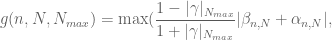
I still haven’t figured out where these patterns are coming from though. I have a vague feeling that one might be able to see things more clearly if one normalises y by dividing it by the factor $\frac{-t}{2} \log \frac{x}{4\pi}$ mentioned previously; it may be that the curved lines one sees in the plots become nearly straight then. (It might be slightly better to use $\frac{x}{4\pi} + \frac{t}{16}$ instead of $\frac{x}{4\pi}$ , though probably the difference is pretty negligible – it’s the difference between the “toy” approximation and the “eff” approximation on the wiki.)

20 December, 2018 at 3:17 pm

Terence Tao

Actually it looks like the correct normalisation is not $y / (-\frac{t}{2} \log \frac{x}{4\pi})$ , but rather $\frac{1}{2} \log \frac{x}{4\pi} + \frac{1+y}{t}$ . It looks like the points on the curves are coming from when adjacent elements in the $\frac{b_n^t}{n^{s_*}}$ series are cancelling each other, thus the points on the outermost curve should be coming from the solutions to the equation

$\displaystyle \frac{b_2^t}{2^{s_*}} = - \frac{b_1^t}{1^{s_*}}$

the second set of points should be coming from

$\displaystyle \frac{b_3^t}{3^{s_*}} = - \frac{b_2^t}{2^{s_*}}$

and so forth. From taking absolute values, then logarithms, it looks like the solutions to

$\displaystyle \frac{b_{n+1}^t}{(n+1)^{s_*}} = - \frac{b_n^t}{n^{s_*}}$

asymptotically lie on the curve

$\displaystyle \frac{1}{2} \log \frac{x}{4\pi} + \frac{1+y}{t} = \frac{1}{2} \log n + \frac{1}{2} \log(n+1)$

or equivalently

$\displaystyle y = \frac{-t}{2} \log \frac{x}{4\pi n(n+1)} - 1$

if I did my calculations correctly (and it seems to fit well with the graphics in your slides). Basically what seems to be happening is that for very large values of y and negative values of t, only two adjacent terms in the B-series dominate, though which two terms dominate depends on exactly where one is in (t,x,y) space, which is where all the different curves come from.

EDIT: the number of zeroes on or near the $n^{th}$ curve up to height $x$ should be approximately $\frac{x}{4\pi} \log \frac{n+1}{n}$ , as compared with the total number of zeroes up to that height, which is about $\frac{x}{4\pi} \log \frac{x}{4\pi}$ .

20 December, 2018 at 4:08 pm

I am sorry for such a naive question: Is your explanation specifically for the zeta function, or generally valid for a large number of functions as a consequence from the heat equation?

20 December, 2018 at 5:22 pm

Terence Tao

From my calculations it seems that this phenomena should occur for any heat flow applied to a Dirichlet series, where the curves are coming from the regions where two adjacent terms in the (heat flowed) Dirichlet series dominate all the other terms, and periodically cancel each other out. This is actually somewhat related to an existing project of one of my graduate students, so I am thinking of getting him to look into this more.

20 December, 2018 at 5:20 pm

Terence Tao

Actually, if these asymptotics can be made rigorous, they should lead to a much simpler proof of the non-negativity $\Lambda \geq 0$ of the de Bruijn-Newman constant, bypassing all the ODE analysis (and also the theory around the pair correlation conjecture) in my paper with Brad. I might get one of my graduate students to look into this further.

21 December, 2018 at 10:16 am

Anonymous

Is it possible to apply such asymptotic to show that a “generalized de Bruijn-Newman constant” is nonnegative for a (possibly large) class of Dirichlet series (e.g. L functions) ?

21 December, 2018 at 4:59 pm

rudolph01

Your formula for the curves fits the patterns of the complex zeros very well ! They seem to even serve like an upper bound on the y-values of the zeros (at least visually up to x=1000).

Curving the zeros

22 December, 2018 at 10:04 am

Terence Tao

Not that it matters too much, but if one uses the eff approximation instead of the toy approximation, one gets the slightly different curves

$\displaystyle \frac{b_n^t}{n^{\mathrm{Re} s_*}} = \frac{b_{n+1}^t}{(n+1)^{\mathrm{Re} s_*}}$

or equivalently

$\displaystyle y = - t (\mathrm{Re} \alpha(\frac{1+y+ix}{2}) - \log \sqrt{n(n+1)}) - 1$

which might be a slightly better fit to the zeroes than the simpler curves described above.

23 December, 2018 at 2:37 pm

rudolph01

Keen to try the eff-approximation, however struggled with the $y$ appearing on both sides of the equation. What would the best way to evaluate such equations?

23 December, 2018 at 6:21 pm

Terence Tao

Iteration should work: start with an initial guess for $y$ (e.g. coming from the toy curve), and insert that in the RHS of the equation for the true curve to obtain a better approximant for y, As the alpha function varies slowly with y, thus should converge very rapidly after just a handful of iterations.

23 December, 2018 at 2:35 pm

rudolph01

We have now some clear indications that the complex zeros organise themselves “into families that peel off the real line at a regular rate”. The question then is what drives the regularity on the ‘peeling off’ process, i.e. what is it that frequently ‘beats the drum’ to start off a new curve of complex zeros, i.e. a new $n, n+1$ -pair starts to dominate at a certain $(x,-t)$ ?

Could this have something to do with the patterns in the real zeros and then in particular with those regular vertical trajectories that don’t seem to originate from a collision between conjugates a ‘long time ago’. When we put $y=0$ in the (toy-model) formula for the n-curves, this yields the following equation:

$x=4 \exp\left(-\frac{2}{t}\right)\pi\,n(n+1)$

Plotting this for $n = 1..6$ gives a set of curves whose spacings seem to match the spacings between these regular vertical trajectories’. It then appears that these originally straight curves have been ‘bended backwards’ by the pressures of the always larger number of real zeros that reside on on their right than on their left. Or is there a much simpler explanation for this?

Although the plot is not quite convincing yet, intuitively these vertical lines seem ideal candidates to serve as the starting point (y=0 case) for an incremental complex curve (next n). The regular patterns in the ‘local minima of complex pair collisions’ between them, are then simply induced by the first, second, etc. zero being ‘born’ on that new curve (going back in time).

These vertical real trajectories seem different from the others. Could there be a way to derive that these vertical lines must have been real forever? If so, then combined with the adage ‘once real, real forever’ and the infinite number of n-curves when $x \rightarrow \infty$ , this might then provide an alternative way to proof Hardy & Littlewood’s theorem that there is an infinite number of zeros on the critical line.

23 December, 2018 at 7:15 pm

Terence Tao

I don’t yet have a good explanation for the unusual patterns at the real axis yet; I am still lacking a plausible and tractable approximation to $H_t(x)$ in this regime (in particular, the approximation that led to the $y = -\frac{t}{2} \log \frac{x}{4\pi n(n+1)} - 1$ curves is completely inaccurate here). Am still working on it. The only thing I have so far is that the variable $x+\pi t/4$ may be slightly better to plot than $x$ (it should straighten all the slanted lines in the plot).

23 December, 2018 at 10:24 pm

Terence Tao

Actually, would it be possible to plot t versus $\sqrt{\frac{x}{4\pi} + \frac{t}{16}}$ for the real zeroes? My calculations are beginning to tell me that the fractional part of $\sqrt{\frac{x}{4\pi} + \frac{t}{16}}$ is somehow relevant (this is essentially the “ $p$ ” quantity in the $C_0(p)$ term of the eff expansion), though I’m not exactly sure how yet. (There’s also something funny going on near the line $\frac{x}{4\pi} + \frac{t}{16} = 0$ that I also don’t understand; I guess the plot I’m asking for only makes sense for the zeroes to the right of this line.)

ADDED LATER: A plot of $t/x$ versus $\sqrt{\frac{x}{4\pi} + \frac{t}{16}}$ might be even more informative (it should make a lot of the diagonal line trends horizontal).

24 December, 2018 at 2:52 am

rudolph01

Here’s the plot.

Lines are indeed straightening out.

24 December, 2018 at 9:10 am

Terence Tao

Thanks! Looks like the long curves arise roughly when $\sqrt{\frac{x}{4\pi} + \frac{t}{16}}$ is close to a half-integer, and the next family of loops come when one is close to an integer. A bit surprised that there is still appreciable drift though, there must be a lower order correction.

I am closing in on a way to plausibly approximate $H_t(x)$ when x is large and t is large and negative (basically by expressing $H_t$ as an integral of the zeta function on the critical line against something roughly gaussian and doing a lot of Taylor expansion and discarding terms which look to be of lower order). This plot will likely be quite helpful in checking the calculations and in suggesting where the most interesting regions of t,x space are. (The calculations are currently incomplete, but I was already seeing the expressions $t/x$ and $\sqrt{\frac{x}{4\pi} + \frac{t}{16}}$ show up a lot, which is why I requested the plot.)

I’m getting hints from the calculations that the theta function might start playing a role. Certainly there is a faint resemblance between the latest plot and some of the imagery at https://en.wikipedia.org/wiki/Theta_function …

24 December, 2018 at 3:20 pm

Terence Tao

Ah, the drift is coming because one should be using

$\displaystyle u:= \frac{|t|}{\frac{x}{4\pi} + \frac{t}{16}}$

as the vertical coordinate rather than t/x. The resulting plot should, I think, be approximately 1-periodic in the horizontal direction; in fact I think that the plot of

$\displaystyle (N,u) := ( \sqrt{\frac{x}{4\pi} + \frac{t}{16}}, \frac{|t|}{\frac{x}{4\pi} + \frac{t}{16}})$

should (assuming I have not made any sign errors) asymptotically coincide with the zeroes of the theta function

$\displaystyle \sum_{n=-\infty}^\infty e^{-\frac{un(n+1)}{16} - \frac{\pi i n(n+1)}{2} + 2\pi i (n+1/2) N} = e^{-\pi i N} \theta_{10}(N, \frac{iu}{16 \pi} - \frac{1}{2} )$
(which one can check to be a real-valued function, 1-periodic in N). I wrote a heuristic derivation of this relationship on the wiki at http://michaelnielsen.org/polymath1/index.php?title=Polymath15_test_problem#Large_negative_values_of_.5Bmath.5Dt.5B.2Fmath.5D . For large values of u, the zeroes should occur when N is close to a half-integer.

24 December, 2018 at 10:03 am

Anonymous

Is it possible that the appearance of theta functions is an indication for the existence of some (still unknown) asymptotic expansion for $H_t(x)$ (where $x, -t$ are large) ?

24 December, 2018 at 3:54 pm

rudolph01

Amazing!

This is the plot I get when using $\frac{|t|}{\frac{x}{4\pi}+\frac{t}{16}}$ instead of $\frac{t}{x}$ . Is this in line with your expectations?

Will start to explore the zeroes of the theta function tomorrow.

24 December, 2018 at 4:30 pm

Terence Tao

Hmm, that’s not what I was expecting at all… oh, wait, the picture is being swamped by the extremely large values of the vertical coordinate. Could you truncate the picture to, say, the right of $\sqrt{\frac{x}{4\pi} + \frac{t}{16}} = 2$ , and rescale? Right now all the interesting behaviour is squashed into the x axis.

25 December, 2018 at 2:02 am

rudolph01

Ah, of course! Sorry for that.

Zoomed in plot (vertical axis values $\le 3.6$ ).

25 December, 2018 at 8:40 am

Terence Tao

Thanks for this! At first I was puzzled as to why the diagram was not as 1-periodic as I had expected, but I think it is because of the numerical cutoffs in t and x which are truncating some of the zero trajectories. (Though it puzzles me somewhat as to why some trajectories are truncated whereas others seem to blast straight through the cutoff.)

25 December, 2018 at 9:12 am

rudolph01

Here is an updated version with the theta zeros as overlay. Looks like a pretty good fit with the straight lines. For calculating the Theta-zeros I used $x = 10...600$ and $t=-200...-1$ (t-steps of 1).

Can’t explain the cut-off’s either yet, but note that exactly the same phenomenon occurs in the Theta-zeros (both lines at 5.5 and 6.5 are shorter). What could happen here is that the t-resolution by which the real zeros of latex H_t$ have been calculated (t-steps of 0.1) are inducing this phenomenon. Will take a deeper dive.

It also seems another asymptotic pattern has emerged in the normalised graph (marked with an arrow). Where could this come from (maybe it is also just caused by the cut-offs)?

25 December, 2018 at 10:06 am

Terence Tao

Hmm, I was expecting the theta function to also capture some of the loops. Is there some way to make a contour plot of theta? It’s complex valued, but the phase is very predictable (it should be $e^{\pi i N}$ , if I have calculated correctly). The theta function should somehow “notice” the loops.

25 December, 2018 at 9:24 am

Anonymous

Is there any quantitative expression for the smooth envelop appearing (with some inner and outer “spikes”) in the plot?

26 December, 2018 at 6:04 am

rudolph01

Getting closer. One mistake I made, is I that used $\sum_{-\infty}^{\infty}$ instead of $\sum_n$ (as in the formula on the wiki-page) to evaluate the Theta-function. I now do get this implicit plot (not normalised) and although the loops do start to get ‘noticed’ they don’t seem to be in the correct spot yet.

26 December, 2018 at 9:57 am

Terence Tao

Hmm, this isn’t as good a fit as I was hoping for, even if one anticipates the presence of sign errors etc. (for instance, it seems that the theta function is not exhibiting enough oscillation near the t=0 axis to account for the interesting behaviour of the zeroes there). But certainly it feels like the approximation is somehow partially correct since it seems to be capturing some, but not all, of the relevant features. I’ll have to think about this some more.

One small thing to try is to use test of the other approximations to $H_t$ that are on the wiki (but note that these approximations are only up to various normalisation factors, so they should capture the zeroes of $H_t$ but not the magnitude). An easy one to start with is the alternate theta function approximation 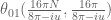$\theta_{01}( \frac{16 \pi N}{8\pi - iu}, \frac{16 \pi}{8\pi - iu})$ . A couple of such plots may help detect any remaining errors either in the wiki derivation or in the numerical implementation.

[ADDED LATER: given the modularity properties of the theta function, I was expecting to see the theta zero set exhibit patterns similar to that of the fundamental domain of the modular group (see e.g. the picture in https://en.wikipedia.org/wiki/Fundamental_domain#Fundamental_domain_for_the_modular_group ), which does resemble somewhat the plots we’re seeing for the zeroes. But something seems to have gone wrong somewhere; not sure what yet.]

26 December, 2018 at 11:07 am

Anonymous

Rudolph, is your theta function evaluation code available? Theta functions are already implemented (acb_modular_theta).

26 December, 2018 at 2:00 pm

rudolph01

Started to work through each asymptotic for $H_t$ on the Wiki and in the section “To cancel off an exponential decay…”, there seems to be something missing in the equation just before “where”.

Shouldn’t $e^{-v^2+\pi\sqrt{|t|}\,v/4}$ be $e^{-v^2+\pi\sqrt{|t|}\,v/4 -\pi^2|t|/64}$ ?

@Anonymous, yes I am aware of the ARB function, however used pari/gp for the current evaluations. Will share the code once I have worked through all the Wiki equations.

26 December, 2018 at 2:31 pm

rudolph01

Ah, ignore my comment: missed the “…we discard any multiplicative factor which is non-zero…” at the beginning!

26 December, 2018 at 4:36 pm

rudolph01

Will continue tomorrow, however did find that I am ‘losing the plot’ between the formula under “is defined in (6) of the writeup” (still ok) and the formula just above “The two factors of” (no longer ok). The strange thing is that when I add the ignored multiplicative factor $M_0((1+i\tilde x)/2)$ back into the integral, the zeros do get closer to the correct ones again (but that shouldn’t happen). Could there be something off in the Taylor expansion step or the achieved accuracy?

26 December, 2018 at 9:07 pm

Terence Tao

I’ve now numbered the equations in the wiki for ease of reference. If I understand what you are saying, then the zeroes of the RHS of (3.7) on the wiki still agree fairly well with the zeroes of $H_t$ , and if one makes the approximation (3.8) then we still have good agreement, but if one makes the approximation (3.9) instead then one no longer has agreement? That suggests some issue with numerical precision (after all, $M_0$ is very small). (Perhaps you are also substituting (3.10) and (3.11) as well, but again this would still sound like a numerical precision issue.)

At any rate, I feel like this sort of numerical walkthrough of the heuristic argument in the wiki should soon pin down exactly where the divergence between theory and numerics is coming from (for instance, we should be able to see which of the approximations (3.8), (3.9), (3.10), (3.11) is somehow faulty). (In the worst case scenario, we might have to explicitly put back in all the non-zero factors that I was dropping to keep the calculations from becoming too messy, as it may be easier to detect the divergence if we have an actual asymptotic rather than just an asymptotic up to non-zero factors).

27 December, 2018 at 2:46 am

Anonymous

Is it possible that the numerical problem appears whenever the nonzero factor of the “main term” of a possible (still unknown) asymptotic expansion of $H_t(x)$ is making the main term “too small” to neglect the influence of the remainder term?

27 December, 2018 at 8:18 am

rudolph01

Thanks for the numbering! Worked through each step and re-injected the multiplicative factors. All went much better numerically, however failed to reconcile the step between 3.16 and 3.17. Could it be that the last $\log{\frac{n}{N}}$ in 3.17 should be $\log{n}$ ?

27 December, 2018 at 2:19 pm

Terence Tao

Hmm, (3.16) and (3.17) should only differ by the constant nonzero multiplicative factor of $N^{\frac{1+i\tilde x}{2}}$ , so I’m at a loss to see what the problem is, perhaps one just has to insert this numerical factor back in again. (It is puzzling though that these factors make so much difference. It must be some numerical computation quirk that I was unaware of.)

27 December, 2018 at 3:45 pm

Anonymous

I’ve tried to reproduce Rudolph’s real zeros plot in https://terrytao.wordpress.com/2018/09/06/polymath15-tenth-thread-numerics-update/#comment-509448 but I got a different looking plot. For each (x, t) in a grid I plotted a blue pixel if theta is negative and a red pixel if theta is positive. This showed four blue and three red diagonal stripes of varying widths, with the six boundary lines between the stripes appearing to correspond to six long straight green lines of Ht zeros in Rudolph’s plot (one of these lines is hard to see in his plot because it’s partly obscured by the legend in the lower left).

27 December, 2018 at 4:53 pm

rudolph01

Still puzzled by the unstable results and probably have made a mistake somewhere but eager to get this sorted. Appreciate any help and have therefore just created a new issue here. It contains the pari/gp code that I have used so far and grateful for any help/hints/tips on where the issue could be!

@anonymous, maybe you could also replicate some equations of the wiki-page in ARB, so we could compare output.

27 December, 2018 at 5:02 pm

Anonymous

print(“eq.328 “,Ht324(1000, -10))

this looks wrong, visually

27 December, 2018 at 6:22 pm

Anonymous

Rudolph, my code is failing the sanity check by not getting a real RHS, so I probably have something wrong in the way I’m calling the theta function or there is a typo on the wiki.

28 December, 2018 at 4:39 am

rudolph01

@anonymous, I am also getting an imaginary part in pari/gp when evaluating the RHS from eq. 3.07 onwards. Therefore don’t think this is induced by incorrect calling of the ARB-theta.

28 December, 2018 at 11:12 am

Polymath 15, eleventh thread: Writing up the results, and exploring negative t | What's new

[…] thread of the Polymath15 project to upper bound the de Bruijn-Newman constant , continuing this post. Discussion of the project of a non-research nature can continue for now in the existing proposal […]

	Dan Asimov on Inequalities, convergence, and…
	Dan Asimov on Inequalities, convergence, and…
	Anonymous on AI to Assist Mathematical Reas…
	Terence Tao on AI to Assist Mathematical Reas…
	Mathur Maynard Amadi on Inequalities, convergence, and…
	Alex Kontorovich on Inequalities, convergence, and…
	Gabe Khan on Inequalities, convergence, and…
	"不等式、收敛与连续性作为“特… on Inequalities, convergence, and…
	Some interesting thi… on PCAST Working Group on Generat…
	jack morava on Inequalities, convergence, and…
	Wednesday assorted l… on Inequalities, convergence, and…
	Wednesday assorted l… on Inequalities, convergence, and…
	Wednesday assorted l… on Inequalities, convergence, and…
	Mark Lewko on Inequalities, convergence, and…
	Wednesday assorted l… on Inequalities, convergence, and…

Polymath15, tenth thread: numerics update

Recent Comments

Articles by others

Diversions

Mathematics

Selected articles

Software

The sciences

Top Posts

Archives

Categories

The Polymath Blog

104 comments

Leave a Reply Cancel reply

For commenters

Polymath15, tenth thread: numerics update

Share this:

Like this:

Recent Comments

Articles by others

Diversions

Mathematics

Selected articles

Software

The sciences

Top Posts

Archives

Categories

The Polymath Blog

104 comments

Leave a Reply Cancel reply

For commenters