The Poincaré upper half-plane 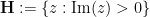 (with a boundary consisting of the real line
  together with the point at infinity
  ) carries an action of the projective special linear group

via fractional linear transformations:

Here and in the rest of the post we will abuse notation by identifying elements  of the special linear group
  with their equivalence class
  in
in  ; this will occasionally create or remove a factor of two in our formulae, but otherwise has very little effect, though one has to check that various definitions and expressions (such as (1)) are unaffected if one replaces a matrix by its negation
  . In particular, we recommend that the reader ignore the signs
  that appear from time to time in the discussion below.
As the action of on  is transitive, and any given point in (e.g.
  ) has a stabiliser isomorphic to the projective rotation group
  , we can view the Poincaré upper half-plane as a homogeneous space for , and more specifically the quotient space of of a maximal compact subgroup . In fact, we can make the half-plane a symmetric space for , by endowing with the Riemannian metric
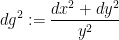
(using Cartesian coordinates  ), which is invariant with respect to the action. Like any other Riemannian metric, the metric on generates a number of other important geometric objects on , such as the distance function
  which can be computed to be given by the formula
the volume measure  , which can be computed to be

and the Laplace-Beltrami operator, which can be computed to be 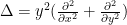 (here we use the negative definite sign convention for
  ). As the metric
  was -invariant, all of these quantities arising from the metric are similarly -invariant in the appropriate sense.
The Gauss curvature of the Poincaré half-plane can be computed to be the constant  , thus is a model for two-dimensional hyperbolic geometry, in much the same way that the unit sphere
  in
in  is a model for two-dimensional spherical geometry (or
  is a model for two-dimensional Euclidean geometry). (Indeed, is isomorphic (via projection to a null hyperplane) to the upper unit hyperboloid
  in the Minkowski spacetime
  , which is the direct analogue of the unit sphere in Euclidean spacetime or the plane in Galilean spacetime
  .)
.)
One can inject arithmetic into this geometric structure by passing from the Lie group to the full modular group
or congruence subgroups such as
for natural number  , or to the discrete stabiliser
  of the point at infinity:
These are discrete subgroups of , nested by the subgroup inclusions

There are many further discrete subgroups of (known collectively as Fuchsian groups) that one could consider, but we will focus attention on these three groups in this post.
Any discrete subgroup  of generates a quotient space
  , which in general will be a non-compact two-dimensional orbifold. One can understand such a quotient space by working with a fundamental domain
  – a set consisting of a single representative of each of the orbits
  of in . This fundamental domain is by no means uniquely defined, but if the fundamental domain is chosen with some reasonable amount of regularity, one can view as the fundamental domain with the boundaries glued together in an appropriate sense. Among other things, fundamental domains can be used to induce a volume measure
  on from the volume measure on (restricted to a fundamental domain). By abuse of notation we will refer to both measures simply as
  when there is no chance of confusion.
For instance, a fundamental domain for  is given (up to null sets) by the strip
  , with identifiable with the cylinder formed by gluing together the two sides of the strip. A fundamental domain for
  is famously given (again up to null sets) by an upper portion
  , with the left and right sides again glued to each other, and the left and right halves of the circular boundary glued to itself. A fundamental domain for
  can be formed by gluing together
![\displaystyle [\hbox{PSL}_2({\bf Z}) : \Gamma_0(q)] = q \prod_{p|q} (1 + \frac{1}{p}) = q^{1+o(1)}](https://s0.wp.com/latex.php?latex=%5Cdisplaystyle++%5B%5Chbox%7BPSL%7D_2%28%7B%5Cbf+Z%7D%29+%3A+%5CGamma_0%28q%29%5D+%3D+q+%5Cprod_%7Bp%7Cq%7D+%281+%2B+%5Cfrac%7B1%7D%7Bp%7D%29+%3D+q%5E%7B1%2Bo%281%29%7D+&bg=ffffff&fg=000000&s=0&c=20201002)
copies of a fundamental domain for in a rather complicated but interesting fashion.
While fundamental domains can be a convenient choice of coordinates to work with for some computations (as well as for drawing appropriate pictures), it is geometrically more natural to avoid working explicitly on such domains, and instead work directly on the quotient spaces . In order to analyse functions  on such orbifolds, it is convenient to lift such functions back up to and identify them with functions
  which are -automorphic in the sense that
  for all
  and
and  . Such functions will be referred to as -automorphic forms, or automorphic forms for short (we always implicitly assume all such functions to be measurable). (Strictly speaking, these are the automorphic forms with trivial factor of automorphy; one can certainly consider other factors of automorphy, particularly when working with holomorphic modular forms, which corresponds to sections of a more non-trivial line bundle over than the trivial bundle
  that is implicitly present when analysing scalar functions . However, we will not discuss this (important) more general situation here.)
An important way to create a -automorphic form is to start with a non-automorphic function obeying suitable decay conditions (e.g. bounded with compact support will suffice) and form the Poincaré series ![{P_\Gamma[f]: {\mathbf H} \rightarrow {\bf C}}](https://s0.wp.com/latex.php?latex=%7BP_%5CGamma%5Bf%5D%3A+%7B%5Cmathbf+H%7D+%5Crightarrow+%7B%5Cbf+C%7D%7D&bg=ffffff&fg=000000&s=0&c=20201002) defined by
defined by
 = \sum_{\gamma \in \Gamma} f(\gamma z),](https://s0.wp.com/latex.php?latex=%5Cdisplaystyle++P_%7B%5CGamma%7D%5Bf%5D%28z%29+%3D+%5Csum_%7B%5Cgamma+%5Cin+%5CGamma%7D+f%28%5Cgamma+z%29%2C&bg=ffffff&fg=000000&s=0&c=20201002)
which is clearly -automorphic. (One could equivalently write  in place of
  here; there are good argument for both conventions, but I have ultimately decided to use the convention, which makes explicit computations a little neater at the cost of making the group actions work in the opposite order.) Thus we naturally see sums over associated with -automorphic forms. A little more generally, given a subgroup of and a -automorphic function of suitable decay, we can form a relative Poincaré series
 ![{P_{\Gamma_\infty \backslash \Gamma}[f]: {\mathbf H} \rightarrow {\bf C}}](https://s0.wp.com/latex.php?latex=%7BP_%7B%5CGamma_%5Cinfty+%5Cbackslash+%5CGamma%7D%5Bf%5D%3A+%7B%5Cmathbf+H%7D+%5Crightarrow+%7B%5Cbf+C%7D%7D&bg=ffffff&fg=000000&s=0&c=20201002) by
by
 = \sum_{\gamma \in \hbox{Fund}(\Gamma_\infty \backslash \Gamma)} f(\gamma z)](https://s0.wp.com/latex.php?latex=%5Cdisplaystyle++P_%7B%5CGamma_%5Cinfty+%5Cbackslash+%5CGamma%7D%5Bf%5D%28z%29+%3D+%5Csum_%7B%5Cgamma+%5Cin+%5Chbox%7BFund%7D%28%5CGamma_%5Cinfty+%5Cbackslash+%5CGamma%29%7D+f%28%5Cgamma+z%29&bg=ffffff&fg=000000&s=0&c=20201002)
where  is any fundamental domain for
  , that is to say a subset of consisting of exactly one representative for each right coset of . As
  is -automorphic, we see (if has suitable decay) that
 ![{P_{\Gamma_\infty \backslash \Gamma}[f]}](https://s0.wp.com/latex.php?latex=%7BP_%7B%5CGamma_%5Cinfty+%5Cbackslash+%5CGamma%7D%5Bf%5D%7D&bg=ffffff&fg=000000&s=0&c=20201002) does not depend on the precise choice of fundamental domain, and is -automorphic. These operations are all compatible with each other, for instance
does not depend on the precise choice of fundamental domain, and is -automorphic. These operations are all compatible with each other, for instance  . A key example of Poincaré series are the Eisenstein series, although there are of course many other Poincaré series one can consider by varying the test function .
For future reference we record the basic but fundamental unfolding identities
![\displaystyle \int_{\Gamma \backslash {\mathbf H}} P_\Gamma[f] g\ d\mu_{\Gamma \backslash {\mathbf H}} = \int_{\mathbf H} f g\ d\mu_{\mathbf H} \ \ \ \ \ (5)](https://s0.wp.com/latex.php?latex=%5Cdisplaystyle++%5Cint_%7B%5CGamma+%5Cbackslash+%7B%5Cmathbf+H%7D%7D+P_%5CGamma%5Bf%5D+g%5C+d%5Cmu_%7B%5CGamma+%5Cbackslash+%7B%5Cmathbf+H%7D%7D+%3D+%5Cint_%7B%5Cmathbf+H%7D+f+g%5C+d%5Cmu_%7B%5Cmathbf+H%7D+%5C+%5C+%5C+%5C+%5C+%285%29&bg=ffffff&fg=000000&s=0&c=20201002)
for any function with sufficient decay, and any -automorphic function  of reasonable growth (e.g. bounded and compact support, and bounded, will suffice). Note that is viewed as a function on on the left-hand side, and as a -automorphic function on on the right-hand side. More generally, one has
![\displaystyle \int_{\Gamma \backslash {\mathbf H}} P_{\Gamma_\infty \backslash \Gamma}[f] g\ d\mu_{\Gamma \backslash {\mathbf H}} = \int_{\Gamma_\infty \backslash {\mathbf H}} f g\ d\mu_{\Gamma_\infty \backslash {\mathbf H}} \ \ \ \ \ (6)](https://s0.wp.com/latex.php?latex=%5Cdisplaystyle++%5Cint_%7B%5CGamma+%5Cbackslash+%7B%5Cmathbf+H%7D%7D+P_%7B%5CGamma_%5Cinfty+%5Cbackslash+%5CGamma%7D%5Bf%5D+g%5C+d%5Cmu_%7B%5CGamma+%5Cbackslash+%7B%5Cmathbf+H%7D%7D+%3D+%5Cint_%7B%5CGamma_%5Cinfty+%5Cbackslash+%7B%5Cmathbf+H%7D%7D+f+g%5C+d%5Cmu_%7B%5CGamma_%5Cinfty+%5Cbackslash+%7B%5Cmathbf+H%7D%7D+%5C+%5C+%5C+%5C+%5C+%286%29&bg=ffffff&fg=000000&s=0&c=20201002)
whenever  are discrete subgroups of , is a -automorphic function with sufficient decay on , and is a -automorphic (and thus also -automorphic) function of reasonable growth. These identities will allow us to move fairly freely between the three domains , , and in our analysis.
When computing various statistics of a Poincaré series ![{P_\Gamma[f]}](https://s0.wp.com/latex.php?latex=%7BP_%5CGamma%5Bf%5D%7D&bg=ffffff&fg=000000&s=0&c=20201002) , such as its values
, such as its values }](https://s0.wp.com/latex.php?latex=%7BP_%5CGamma%5Bf%5D%28z%29%7D&bg=ffffff&fg=000000&s=0&c=20201002) at special points
at special points  , or the
  quantity
 ![{\int_{\Gamma \backslash {\mathbf H}} |P_\Gamma[f]|^2\ d\mu}](https://s0.wp.com/latex.php?latex=%7B%5Cint_%7B%5CGamma+%5Cbackslash+%7B%5Cmathbf+H%7D%7D+%7CP_%5CGamma%5Bf%5D%7C%5E2%5C+d%5Cmu%7D&bg=ffffff&fg=000000&s=0&c=20201002) , expressions of interest to analytic number theory naturally emerge. We list three basic examples of this below, discussed somewhat informally in order to highlight the main ideas rather than the technical details.
, expressions of interest to analytic number theory naturally emerge. We list three basic examples of this below, discussed somewhat informally in order to highlight the main ideas rather than the technical details.
The first example we will give concerns the problem of estimating the sum
where  is the divisor function. This can be rewritten (by factoring
  and
and  ) as
) as
which is basically a sum over the full modular group  . At this point we will “cheat” a little by moving to the related, but different, sum
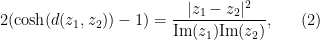
This sum is not exactly the same as (8), but will be a little easier to handle, and it is plausible that the methods used to handle this sum can be modified to handle (8). Observe from (2) and some calculation that the distance between and  is given by the formula
and so one can express the above sum as

(the factor of  coming from the quotient by
  in the projective special linear group); one can express this as
 }](https://s0.wp.com/latex.php?latex=%7BP_%5CGamma%5Bf%5D%28i%29%7D&bg=ffffff&fg=000000&s=0&c=20201002) , where
, where  and is the indicator function of the ball
  . Thus we see that expressions such as (7) are related to evaluations of Poincaré series. (In practice, it is much better to use smoothed out versions of indicator functions in order to obtain good control on sums such as (7) or (9), but we gloss over this technical detail here.)
The second example concerns the relative

of the sum (7). Note from multiplicativity that (7) can be written as  , which is superficially very similar to (10), but with the key difference that the polynomial
  is irreducible over the integers.
As with (7), we may expand (10) as
At first glance this does not look like a sum over a modular group, but one can manipulate this expression into such a form in one of two (closely related) ways. First, observe that any factorisation  of
of  into Gaussian integers
  gives rise (upon taking norms) to an identity of the form
  , where
  and
and  . Conversely, by using the unique factorisation of the Gaussian integers, every identity of the form
  gives rise to a factorisation of the form
  , essentially uniquely up to units. Now note that
  is of the form if and only if
  , in which case
  . Thus we can essentially write the above sum as something like

and one the modular group is now manifest. An equivalent way to see these manipulations is as follows. A triple  of natural numbers with
  gives rise to a positive quadratic form
  of normalised discriminant
  equal to with integer coefficients (it is natural here to allow
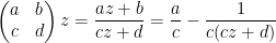
  to take integer values rather than just natural number values by essentially doubling the sum). The group acts on the space of such quadratic forms in a natural fashion (by composing the quadratic form with the inverse
  of an element of
  ). Because the discriminant has class number one (this fact is equivalent to the unique factorisation of the gaussian integers, as discussed in this previous post), every form
  in this space is equivalent (under the action of some element of ) with the standard quadratic form
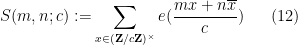
  . In other words, one has

which (up to a harmless sign) is exactly the representation ,  ,
,  introduced earlier, and leads to the same reformulation of the sum (10) in terms of expressions like (11). Similar considerations also apply if the quadratic polynomial is replaced by another quadratic, although one has to account for the fact that the class number may now exceed one (so that unique factorisation in the associated quadratic ring of integers breaks down), and in the positive discriminant case the fact that the group of units might be infinite presents another significant technical problem.
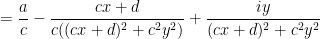
Note that has real part  and imaginary part
  . Thus (11) is (up to a factor of two) the Poincaré series as in the preceding example, except that is now the indicator of the sector
  .
.
Sums involving subgroups of the full modular group, such as  , often arise when imposing congruence conditions on sums such as (10), for instance when trying to estimate the expression
  when and
  are large. As before, one then soon arrives at the problem of evaluating a Poincaré series at one or more special points, where the series is now over rather than .
The third and final example concerns averages of Kloosterman sums
where  and
and  is the inverse of in the multiplicative group
  . It turns out that the norms of Poincaré series or are closely tied to such averages. Consider for instance the quantity
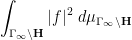
![\displaystyle \int_{\Gamma_0(q) \backslash {\mathbf H}} |P_{\Gamma_\infty \backslash \Gamma_0(q)}[f]|^2\ d\mu_{\Gamma \backslash {\mathbf H}} \ \ \ \ \ (13)](https://s0.wp.com/latex.php?latex=%5Cdisplaystyle++%5Cint_%7B%5CGamma_0%28q%29+%5Cbackslash+%7B%5Cmathbf+H%7D%7D+%7CP_%7B%5CGamma_%5Cinfty+%5Cbackslash+%5CGamma_0%28q%29%7D%5Bf%5D%7C%5E2%5C+d%5Cmu_%7B%5CGamma+%5Cbackslash+%7B%5Cmathbf+H%7D%7D+%5C+%5C+%5C+%5C+%5C+%2813%29&bg=ffffff&fg=000000&s=0&c=20201002)
where is a natural number and is a -automorphic form that is of the form

for some integer  and some test function
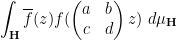
  , which for sake of discussion we will take to be smooth and compactly supported. Using the unfolding formula (6), we may rewrite (13) as
![\displaystyle \int_{\Gamma_\infty \backslash {\mathbf H}} \overline{f} P_{\Gamma_\infty \backslash \Gamma_0(q)}[f]\ d\mu_{\Gamma_\infty \backslash {\mathbf H}}.](https://s0.wp.com/latex.php?latex=%5Cdisplaystyle++%5Cint_%7B%5CGamma_%5Cinfty+%5Cbackslash+%7B%5Cmathbf+H%7D%7D+%5Coverline%7Bf%7D+P_%7B%5CGamma_%5Cinfty+%5Cbackslash+%5CGamma_0%28q%29%7D%5Bf%5D%5C+d%5Cmu_%7B%5CGamma_%5Cinfty+%5Cbackslash+%7B%5Cmathbf+H%7D%7D.&bg=ffffff&fg=000000&s=0&c=20201002)
To compute this, we use the double coset decomposition
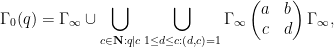
where for each  ,
,  are arbitrarily chosen integers such that . To see this decomposition, observe that every element in outside of can be assumed to have
  by applying a sign , and then using the row and column operations coming from left and right multiplication by (that is, shifting the top row by an integer multiple of the bottom row, and shifting the right column by an integer multiple of the left column) one can place
  in the interval
 ![{[1,c]}](https://s0.wp.com/latex.php?latex=%7B%5B1%2Cc%5D%7D&bg=ffffff&fg=000000&s=0&c=20201002) and
and  to be any specified integer pair with . From this we see that
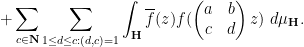
![\displaystyle P_{\Gamma_\infty \backslash \Gamma_0(q)}[f] = f + \sum_{c \in {\mathbf N}: q|c} \sum_{1 \leq d \leq c: (d,c)=1} P_{\Gamma_\infty}[ f( \begin{pmatrix} a & b \\ c & d \end{pmatrix} \cdot ) ]](https://s0.wp.com/latex.php?latex=%5Cdisplaystyle++P_%7B%5CGamma_%5Cinfty+%5Cbackslash+%5CGamma_0%28q%29%7D%5Bf%5D+%3D+f+%2B+%5Csum_%7Bc+%5Cin+%7B%5Cmathbf+N%7D%3A+q%7Cc%7D+%5Csum_%7B1+%5Cleq+d+%5Cleq+c%3A+%28d%2Cc%29%3D1%7D+P_%7B%5CGamma_%5Cinfty%7D%5B+f%28+%5Cbegin%7Bpmatrix%7D+a+%26+b+%5C%5C+c+%26+d+%5Cend%7Bpmatrix%7D+%5Ccdot+%29+%5D&bg=ffffff&fg=000000&s=0&c=20201002)
and so from further use of the unfolding formula (5) we may expand (13) as
The first integral is just  . The second expression is more interesting. We have
so we can write
as


which on shifting by  simplifies a little to


and then on scaling  by simplifies a little further to

Note that as , we have  modulo
  . Comparing the above calculations with (12), we can thus write (13) as
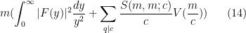
where

is a certain integral involving  and a parameter
  , but which does not depend explicitly on parameters such as
  . Thus we have indeed expressed the expression (13) in terms of Kloosterman sums. It is possible to invert this analysis and express varius weighted sums of Kloosterman sums in terms of expressions (possibly involving inner products instead of norms) of Poincaré series, but we will not do so here; see Chapter 16 of Iwaniec and Kowalski for further details.
Traditionally, automorphic forms have been analysed using the spectral theory of the Laplace-Beltrami operator  on spaces such as
  or , so that a Poincaré series such as might be expanded out using inner products of (or, by the unfolding identities, ) with various generalised eigenfunctions of (such as cuspidal eigenforms, or Eisenstein series). With this approach, special functions, and specifically the modified Bessel functions
  of the second kind, play a prominent role, basically because the -automorphic functions

for  and
and  non-zero are generalised eigenfunctions of (with eigenvalue
  ), and are almost square-integrable on (the norm diverges only logarithmically at one end
  of the cylinder , while decaying exponentially fast at the other end
  ).
).
However, as discussed in this previous post, the spectral theory of an essentially self-adjoint operator such as is basically equivalent to the theory of various solution operators associated to partial differential equations involving that operator, such as the Helmholtz equation  , the heat equation
  , the Schrödinger equation
 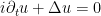 , or the wave equation
  . Thus, one can hope to rephrase many arguments that involve spectral data of into arguments that instead involve resolvents
  , heat kernels
  , Schrödinger propagators
  , or wave propagators
  , or involve the PDE more directly (e.g. applying integration by parts and energy methods to solutions of such PDE). This is certainly done to some extent in the existing literature; resolvents and heat kernels, for instance, are often utilised. In this post, I would like to explore the possibility of reformulating spectral arguments instead using the inhomogeneous wave equation

Actually it will be a bit more convenient to normalise the Laplacian by  , and look instead at the automorphic wave equation

This equation somewhat resembles a “Klein-Gordon” type equation, except that the mass is imaginary! This would lead to pathological behaviour were it not for the negative curvature, which in principle creates a spectral gap of that cancels out this factor.
The point is that the wave equation approach gives access to some nice PDE techniques, such as energy methods, Sobolev inequalities and finite speed of propagation, which are somewhat submerged in the spectral framework. The wave equation also interacts well with Poincaré series; if for instance and are -automorphic solutions to (15) obeying suitable decay conditions, then their Poincaré series ![{P_{\Gamma_\infty \backslash \Gamma}[u]}](https://s0.wp.com/latex.php?latex=%7BP_%7B%5CGamma_%5Cinfty+%5Cbackslash+%5CGamma%7D%5Bu%5D%7D&bg=ffffff&fg=000000&s=0&c=20201002) and
and ![{P_{\Gamma_\infty \backslash \Gamma}[F]}](https://s0.wp.com/latex.php?latex=%7BP_%7B%5CGamma_%5Cinfty+%5Cbackslash+%5CGamma%7D%5BF%5D%7D&bg=ffffff&fg=000000&s=0&c=20201002) will be -automorphic solutions to the same equation (15), basically because the Laplace-Beltrami operator commutes with translations. Because of these facts, it is possible to replicate several standard spectral theory arguments in the wave equation framework, without having to deal directly with things like the asymptotics of modified Bessel functions. The wave equation approach to automorphic theory was introduced by Faddeev and Pavlov (using the Lax-Phillips scattering theory), and developed further by by Lax and Phillips, to recover many spectral facts about the Laplacian on modular curves, such as the Weyl law and the Selberg trace formula. Here, I will illustrate this by deriving three basic applications of automorphic methods in a wave equation framework, namely
will be -automorphic solutions to the same equation (15), basically because the Laplace-Beltrami operator commutes with translations. Because of these facts, it is possible to replicate several standard spectral theory arguments in the wave equation framework, without having to deal directly with things like the asymptotics of modified Bessel functions. The wave equation approach to automorphic theory was introduced by Faddeev and Pavlov (using the Lax-Phillips scattering theory), and developed further by by Lax and Phillips, to recover many spectral facts about the Laplacian on modular curves, such as the Weyl law and the Selberg trace formula. Here, I will illustrate this by deriving three basic applications of automorphic methods in a wave equation framework, namely
- Using the Weil bound on Kloosterman sums to derive Selberg’s 3/16 theorem on the least non-trivial eigenvalue for on (discussed previously here);
- Conversely, showing that Selberg’s eigenvalue conjecture (improving Selberg’s
 bound to the optimal
  ) implies an optimal bound on (smoothed) sums of Kloosterman sums; and
- Using the same bound to obtain pointwise bounds on Poincaré series similar to the ones discussed above. (Actually, the argument here does not use the wave equation, instead it just uses the Sobolev inequality.)
This post originated from an attempt to finally learn this part of analytic number theory properly, and to see if I could use a PDE-based perspective to understand it better. Ultimately, this is not that dramatic a depature from the standard approach to this subject, but I found it useful to think of things in this fashion, probably due to my existing background in PDE.
I thank Bill Duke and Ben Green for helpful discussions. My primary reference for this theory was Chapters 15, 16, and 21 of Iwaniec and Kowalski.
Read the rest of this entry »


Recent Comments