Tag Archive

You are currently browsing the tag archive for the ‘binomial coefficients’ tag.

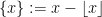
Singmaster’s conjecture in the interior of Pascal’s triangle

7 June, 2021 in math.NT, paper | Tags: binomial coefficients, exponential sums, Joni Teravainen, Kaisa Matomaki, Maksym Radziwill, Singmaster's conjecture, Xuancheng Shao | by Terence Tao | 31 comments

Kaisa Matomäki, Maksym Radziwill, Xuancheng Shao, Joni Teräväinen, and myself have just uploaded to the arXiv our preprint “Singmaster’s conjecture in the interior of Pascal’s triangle“. This paper leverages the theory of exponential sums over primes to make progress on a well known conjecture of Singmaster which asserts that any natural number larger than ${1}$ appears at most a bounded number of times in Pascal’s triangle. That is to say, for any integer ${t \geq 2}$ , there are at most ${O(1)}$ solutions to the equation

$\displaystyle \binom{n}{m} = t \ \ \ \ \ (1)$

with ${1 \leq m < n}$ . Currently, the largest number of solutions that is known to be attainable is eight, with ${t}$ equal to

$\displaystyle 3003 = \binom{3003}{1} = \binom{78}{2} = \binom{15}{5} = \binom{14}{6} = \binom{14}{8} = \binom{15}{10}$

$\displaystyle = \binom{78}{76} = \binom{3003}{3002}.$

Because of the symmetry ${\binom{n}{m} = \binom{n}{n-m}}$ of Pascal’s triangle it is natural to restrict attention to the left half ${1 \leq m \leq n/2}$ of the triangle.

Our main result settles this conjecture in the “interior” region of the triangle:

Theorem 1 (Singmaster’s conjecture in the interior of the triangle) If ${0 < \varepsilon < 1}$ and ${t}$ is sufficiently large depending on ${\varepsilon}$ , there are at most two solutions to (1) in the region
$\displaystyle \exp( \log^{2/3+\varepsilon} n ) \leq m \leq n/2 \ \ \ \ \ (2)$
and hence at most four in the region
$\displaystyle \exp( \log^{2/3+\varepsilon} n ) \leq m \leq n - \exp( \log^{2/3+\varepsilon} n ).$
Also, there is at most one solution in the region
$\displaystyle \exp( \log^{2/3+\varepsilon} n ) \leq m \leq n/\exp(\log^{1-\varepsilon} n ).$

To verify Singmaster’s conjecture in full, it thus suffices in view of this result to verify the conjecture in the boundary region

$\displaystyle 2 \leq m < \exp(\log^{2/3+\varepsilon} n) \ \ \ \ \ (3)$

(or equivalently ${n - \exp(\log^{2/3+\varepsilon} n) < m \leq n}$ ); we have deleted the ${m=1}$ case as it of course automatically supplies exactly one solution to (1). It is in fact possible that for ${t}$ sufficiently large there are no further collisions ${\binom{n}{m} = \binom{n'}{m'}=t}$ for ${(n,m), (n',m')}$ in the region (3), in which case there would never be more than eight solutions to (1) for sufficiently large ${t}$ . This is latter claim known for bounded values of ${m,m'}$ by Beukers, Shorey, and Tildeman, with the main tool used being Siegel’s theorem on integral points.

The upper bound of two here for the number of solutions in the region (2) is best possible, due to the infinite family of solutions to the equation

$\displaystyle \binom{n+1}{m+1} = \binom{n}{m+2} \ \ \ \ \ (4)$

coming from ${n = F_{2j+2} F_{2j+3}-1}$ , ${m = F_{2j} F_{2j+3}-1}$ and ${F_j}$ is the ${j^{th}}$ Fibonacci number.

The appearance of the quantity ${\exp( \log^{2/3+\varepsilon} n )}$ in Theorem 1 may be familiar to readers that are acquainted with Vinogradov’s bounds on exponential sums, which ends up being the main new ingredient in our arguments. In principle this threshold could be lowered if we had stronger bounds on exponential sums.

To try to control solutions to (1) we use a combination of “Archimedean” and “non-Archimedean” approaches. In the “Archimedean” approach (following earlier work of Kane on this problem) we view ${n,m}$ primarily as real numbers rather than integers, and express (1) in terms of the Gamma function as

$\displaystyle \frac{\Gamma(n+1)}{\Gamma(m+1) \Gamma(n-m+1)} = t.$

One can use this equation to solve for ${n}$ in terms of ${m,t}$ as

$\displaystyle n = f_t(m)$

for a certain real analytic function ${f_t}$ whose asymptotics are easily computable (for instance one has the asymptotic ${f_t(m) \asymp m t^{1/m}}$ ). One can then view the problem as one of trying to control the number of lattice points on the graph ${\{ (m,f_t(m)): m \in {\bf R} \}}$ . Here we can take advantage of the fact that in the regime ${m \leq f_t(m)/2}$ (which corresponds to working in the left half ${m \leq n/2}$ of Pascal’s triangle), the function ${f_t}$ can be shown to be convex, but not too convex, in the sense that one has both upper and lower bounds on the second derivative of ${f_t}$ (in fact one can show that ${f''_t(m) \asymp f_t(m) (\log t/m^2)^2}$ ). This can be used to preclude the possibility of having a cluster of three or more nearby lattice points on the graph ${\{ (m,f_t(m)): m \in {\bf R} \}}$ , basically because the area subtended by the triangle connecting three of these points would lie between ${0}$ and ${1/2}$ , contradicting Pick’s theorem. Developing these ideas, we were able to show

Proposition 2 Let ${\varepsilon>0}$ , and suppose ${t}$ is sufficiently large depending on ${\varepsilon}$ . If ${(m,n)}$ is a solution to (1) in the left half ${m \leq n/2}$ of Pascal’s triangle, then there is at most one other solution ${(m',n')}$ to this equation in the left half with
$\displaystyle |m-m'| + |n-n'| \ll \exp( (\log\log t)^{1-\varepsilon} ).$

Again, the example of (4) shows that a cluster of two solutions is certainly possible; the convexity argument only kicks in once one has a cluster of three or more solutions.

To finish the proof of Theorem 1, one has to show that any two solutions ${(m,n), (m',n')}$ to (1) in the region of interest must be close enough for the above proposition to apply. Here we switch to the “non-Archimedean” approach, in which we look at the ${p}$ -adic valuations ${\nu_p( \binom{n}{m} )}$ of the binomial coefficients, defined as the number of times a prime ${p}$ divides ${\binom{n}{m}}$ . From the fundamental theorem of arithmetic, a collision

$\displaystyle \binom{n}{m} = \binom{n'}{m'}$

between binomial coefficients occurs if and only if one has agreement of valuations

$\displaystyle \nu_p( \binom{n}{m} ) = \nu_p( \binom{n'}{m'} ). \ \ \ \ \ (5)$

From the Legendre formula

$\displaystyle \nu_p(n!) = \sum_{j=1}^\infty \lfloor \frac{n}{p^j} \rfloor$

we can rewrite this latter identity (5) as

$\displaystyle \sum_{j=1}^\infty \{ \frac{m}{p^j} \} + \{ \frac{n-m}{p^j} \} - \{ \frac{n}{p^j} \} = \sum_{j=1}^\infty \{ \frac{m'}{p^j} \} + \{ \frac{n'-m'}{p^j} \} - \{ \frac{n'}{p^j} \}, \ \ \ \ \ (6)$

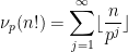
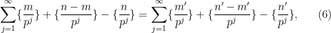
where ${\{x\} := x - \lfloor x\rfloor}$ denotes the fractional part of ${x}$ . (These sums are not truly infinite, because the summands vanish once ${p^j}$ is larger than ${\max(n,n')}$ .)

A key idea in our approach is to view this condition (6) statistically, for instance by viewing ${p}$ as a prime drawn randomly from an interval such as ${[P, P + P \log^{-100} P]}$ for some suitably chosen scale parameter ${P}$ , so that the two sides of (6) now become random variables. It then becomes advantageous to compare correlations between these two random variables and some additional test random variable. For instance, if ${n}$ and ${n'}$ are far apart from each other, then one would expect the left-hand side of (6) to have a higher correlation with the fractional part ${\{ \frac{n}{p}\}}$ , since this term shows up in the summation on the left-hand side but not the right. Similarly if ${m}$ and ${m'}$ are far apart from each other (although there are some annoying cases one has to treat separately when there is some “unexpected commensurability”, for instance if ${n'-m'}$ is a rational multiple of ${m}$ where the rational has bounded numerator and denominator). In order to execute this strategy, it turns out (after some standard Fourier expansion) that one needs to get good control on exponential sums such as

$\displaystyle \sum_{P \leq p \leq P + P\log^{-100} P} e( \frac{N}{p} + \frac{M}{p^j} )$

for various choices of parameters ${P, N, M, j}$ , where ${e(\theta) := e^{2\pi i \theta}}$ . Fortunately, the methods of Vinogradov (which more generally can handle sums such as ${\sum_{n \in I} e(f(n))}$ and ${\sum_{p \in I} e(f(p))}$ for various analytic functions ${f}$ ) can give useful bounds on such sums as long as ${N}$ and ${M}$ are not too large compared to ${P}$ ; more specifically, Vinogradov’s estimates are non-trivial in the regime ${N,M \ll \exp( \log^{3/2-\varepsilon} P )}$ , and this ultimately leads to a distance bound

$\displaystyle m' - m \ll_\varepsilon \exp( \log^{2/3 +\varepsilon}(n+n') )$

between any colliding pair ${(n,m), (n',m')}$ in the left half of Pascal’s triangle, as well as the variant bound

$\displaystyle n' - n \ll_\varepsilon \exp( \log^{2/3 +\varepsilon}(n+n') )$

under the additional assumption

$\displaystyle m', m \geq \exp( \log^{2/3 +\varepsilon}(n+n') ).$

Comparing these bounds with Proposition 2 and using some basic estimates about the function ${f_t}$ , we can conclude Theorem 1.

A modification of the arguments also gives similar results for the equation

$\displaystyle (n)_m = t \ \ \ \ \ (7)$

where ${(n)_m := n (n-1) \dots (n-m+1)}$ is the falling factorial:

Theorem 3 If ${0 < \varepsilon < 1}$ and ${t}$ is sufficiently large depending on ${\varepsilon}$ , there are at most two solutions to (7) in the region
$\displaystyle \exp( \log^{2/3+\varepsilon} n ) \leq m < n. \ \ \ \ \ (8)$

Again the upper bound of two is best possible, thanks to identities such as

$\displaystyle (a^2-a)_{a^2-2a} = (a^2-a-1)_{a^2-2a+1}.$

Conversions between standard polynomial bases

7 April, 2019 in expository, math.CO, math.RA | Tags: binomial coefficients, Eulerian numbers, polynomials, Stirling numbers | by Terence Tao | 24 comments

(This post is mostly intended for my own reference, as I found myself repeatedly looking up several conversions between polynomial bases on various occasions.)

Let ${\mathrm{Poly}_{\leq n}}$ denote the vector space of polynomials ${P:{\bf R} \rightarrow {\bf R}}$ of one variable ${x}$ with real coefficients of degree at most ${n}$ . This is a vector space of dimension ${n+1}$ , and the sequence of these spaces form a filtration:

$\displaystyle \mathrm{Poly}_{\leq 0} \subset \mathrm{Poly}_{\leq 1} \subset \mathrm{Poly}_{\leq 2} \subset \dots$

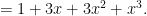
A standard basis for these vector spaces are given by the monomials ${x^0, x^1, x^2, \dots}$ : every polynomial ${P(x)}$ in ${\mathrm{Poly}_{\leq n}}$ can be expressed uniquely as a linear combination of the first ${n+1}$ monomials ${x^0, x^1, \dots, x^n}$ . More generally, if one has any sequence ${Q_0(x), Q_1(x), Q_2(x)}$ of polynomials, with each ${Q_n}$ of degree exactly ${n}$ , then an easy induction shows that ${Q_0(x),\dots,Q_n(x)}$ forms a basis for ${\mathrm{Poly}_{\leq n}}$ .

In particular, if we have two such sequences ${Q_0(x), Q_1(x), Q_2(x),\dots}$ and ${R_0(x), R_1(x), R_2(x), \dots}$ of polynomials, with each ${Q_n}$ of degree ${n}$ and each ${R_k}$ of degree ${k}$ , then ${Q_n}$ must be expressible uniquely as a linear combination of the polynomials ${R_0,R_1,\dots,R_n}$ , thus we have an identity of the form

$\displaystyle Q_n(x) = \sum_{k=0}^n c_{QR}(n,k) R_k(x)$

for some change of basis coefficients ${c_{QR}(n,k) \in {\bf R}}$ . These coefficients describe how to convert a polynomial expressed in the ${Q_n}$ basis into a polynomial expressed in the ${R_k}$ basis.

Many standard combinatorial quantities ${c(n,k)}$ involving two natural numbers ${0 \leq k \leq n}$ can be interpreted as such change of basis coefficients. The most familiar example are the binomial coefficients ${\binom{n}{k}}$ , which measures the conversion from the shifted monomial basis ${(x+1)^n}$ to the monomial basis ${x^k}$ , thanks to (a special case of) the binomial formula:

$\displaystyle (x+1)^n = \sum_{k=0}^n \binom{n}{k} x^k,$

thus for instance

$\displaystyle (x+1)^3 = \binom{3}{0} x^0 + \binom{3}{1} x^1 + \binom{3}{2} x^2 + \binom{3}{3} x^3$

$\displaystyle = 1 + 3x + 3x^2 + x^3.$

More generally, for any shift ${h}$ , the conversion from ${(x+h)^n}$ to ${x^k}$ is measured by the coefficients ${h^{n-k} \binom{n}{k}}$ , thanks to the general case of the binomial formula.

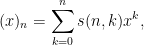
But there are other bases of interest too. For instance if one uses the falling factorial basis

$\displaystyle (x)_n := x (x-1) \dots (x-n+1)$

then the conversion from falling factorials to monomials is given by the Stirling numbers of the first kind ${s(n,k)}$ :

$\displaystyle (x)_n = \sum_{k=0}^n s(n,k) x^k,$

thus for instance

$\displaystyle (x)_3 = s(3,0) x^0 + s(3,1) x^1 + s(3,2) x^2 + s(3,3) x^3$

$\displaystyle = 0 + 2 x - 3x^2 + x^3$

and the conversion back is given by the Stirling numbers of the second kind ${S(n,k)}$ :

$\displaystyle x^n = \sum_{k=0}^n S(n,k) (x)_k$

thus for instance

$\displaystyle x^3 = S(3,0) (x)_0 + S(3,1) (x)_1 + S(3,2) (x)_2 + S(3,3) (x)_3$

$\displaystyle = 0 + x + 3 x(x-1) + x(x-1)(x-2).$

If one uses the binomial functions ${\binom{x}{n} = \frac{1}{n!} (x)_n}$ as a basis instead of the falling factorials, one of course can rewrite these conversions as

$\displaystyle \binom{x}{n} = \sum_{k=0}^n \frac{1}{n!} s(n,k) x^k$

and

$\displaystyle x^n = \sum_{k=0}^n k! S(n,k) \binom{x}{k}$

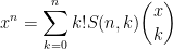
thus for instance

$\displaystyle \binom{x}{3} = 0 + \frac{1}{3} x - \frac{1}{2} x^2 + \frac{1}{6} x^3$

and

$\displaystyle x^3 = 0 + \binom{x}{1} + 6 \binom{x}{2} + 6 \binom{x}{3}.$

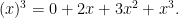
As a slight variant, if one instead uses rising factorials

$\displaystyle (x)^n := x (x+1) \dots (x+n-1)$

then the conversion to monomials yields the unsigned Stirling numbers ${|s(n,k)|}$ of the first kind:

$\displaystyle (x)^n = \sum_{k=0}^n |s(n,k)| x^k$

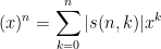
thus for instance

$\displaystyle (x)^3 = 0 + 2x + 3x^2 + x^3.$

One final basis comes from the polylogarithm functions

$\displaystyle \mathrm{Li}_{-n}(x) := \sum_{j=1}^\infty j^n x^j.$

For instance one has

$\displaystyle \mathrm{Li}_1(x) = -\log(1-x)$

$\displaystyle \mathrm{Li}_0(x) = \frac{x}{1-x}$

$\displaystyle \mathrm{Li}_{-1}(x) = \frac{x}{(1-x)^2}$

$\displaystyle \mathrm{Li}_{-2}(x) = \frac{x}{(1-x)^3} (1+x)$

$\displaystyle \mathrm{Li}_{-3}(x) = \frac{x}{(1-x)^4} (1+4x+x^2)$

$\displaystyle \mathrm{Li}_{-4}(x) = \frac{x}{(1-x)^5} (1+11x+11x^2+x^3)$

and more generally one has

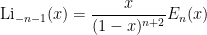
$\displaystyle \mathrm{Li}_{-n-1}(x) = \frac{x}{(1-x)^{n+2}} E_n(x)$

for all natural numbers ${n}$ and some polynomial ${E_n}$ of degree ${n}$ (the Eulerian polynomials), which when converted to the monomial basis yields the (shifted) Eulerian numbers

$\displaystyle E_n(x) = \sum_{k=0}^n A(n+1,k) x^k.$

For instance

$\displaystyle E_3(x) = A(4,0) x^0 + A(4,1) x^1 + A(4,2) x^2 + A(4,3) x^3$

$\displaystyle = 1 + 11x + 11x^2 + x^3.$

These particular coefficients also have useful combinatorial interpretations. For instance:

The binomial coefficient ${\binom{n}{k}}$ is of course the number of ${k}$ -element subsets of ${\{1,\dots,n\}}$ .
The unsigned Stirling numbers ${|s(n,k)|}$ of the first kind are the number of permutations of ${\{1,\dots,n\}}$ with exactly ${k}$ cycles. The signed Stirling numbers ${s(n,k)}$ are then given by the formula ${s(n,k) = (-1)^{n-k} |s(n,k)|}$ .
The Stirling numbers ${S(n,k)}$ of the second kind are the number of ways to partition ${\{1,\dots,n\}}$ into ${k}$ non-empty subsets.
The Eulerian numbers ${A(n,k)}$ are the number of permutations of ${\{1,\dots,n\}}$ with exactly ${k}$ ascents.

These coefficients behave similarly to each other in several ways. For instance, the binomial coefficients ${\binom{n}{k}}$ obey the well known Pascal identity

$\displaystyle \binom{n+1}{k} = \binom{n}{k} + \binom{n}{k-1}$

(with the convention that ${\binom{n}{k}}$ vanishes outside of the range ${0 \leq k \leq n}$ ). In a similar spirit, the unsigned Stirling numbers ${|s(n,k)|}$ of the first kind obey the identity

$\displaystyle |s(n+1,k)| = n |s(n,k)| + |s(n,k-1)|$

and the signed counterparts ${s(n,k)}$ obey the identity

$\displaystyle s(n+1,k) = -n s(n,k) + s(n,k-1).$

The Stirling numbers of the second kind ${S(n,k)}$ obey the identity

$\displaystyle S(n+1,k) = k S(n,k) + S(n,k-1)$

and the Eulerian numbers ${A(n,k)}$ obey the identity

$\displaystyle A(n+1,k) = (k+1) A(n,k) + (n-k+1) A(n,k-1).$

	Anonymous on Erratum for “An inverse…
	Anonymous on Infinite partial sumsets in th…
	Anonymous on Infinite partial sumsets in th…
	Anonymous on A Banach algebra proof of the…
	Anonymous on A Banach algebra proof of the…
	Aleksandar on 245C, Notes 4: Sobolev sp…
	Anonymous on Erratum for “An inverse…
	Anonymous on Erratum for “An inverse…
	Anonymous on Erratum for “An inverse…
	Anonymous on Erratum for “An inverse…
	Terence Tao on 245C, Notes 4: Sobolev sp…
	Terence Tao on 275A, Notes 3: The weak and st…
	Terence Tao on What is a gauge?
	Terence Tao on Erratum for “An inverse…
	Terence Tao on 275A, Notes 3: The weak and st…

Tag Archive

Singmaster’s conjecture in the interior of Pascal’s triangle

Conversions between standard polynomial bases

Recent Comments

Articles by others

Diversions

Mathematics

Selected articles

Software

The sciences

Top Posts

Archives

Categories

The Polymath Blog

For commenters