We now turn to Perelman’s second scale-invariant monotone quantity for Ricci flow, now known as the Perelman reduced volume. We saw in the previous lecture that the monotonicity for Perelman entropy was ultimately derived (after some twists and turns) from the monotonicity of a potential under gradient flow. In this lecture, we will show (at a heuristic level only) how the monotonicity of Perelman’s reduced volume can also be “derived”, in a formal sense, from another source of monotonicity, namely the relative Bishop-Gromov inequality in comparison geometry (which has already been alluded to in previous lectures). Interestingly, in order to obtain this connection, one must first reinterpret parabolic flows such as Ricci flow as the limit of a certain high-dimensional Riemannian manifold as the dimension becomes infinite; this is part of a more general philosophy that parabolic theory is in some sense an infinite-dimensional limit of elliptic theory. Our treatment here is a (liberally reinterpreted) version of Section 6 of Perelman’s paper.
In the next few lectures we shall give a rigorous proof of this monotonicity, without using the infinite-dimensional limit and instead using results related to the Li-Yau-Hamilton Harnack inequality. (There are several other approaches to understanding Perelman’s reduced volume, such as Lott’s formulation based on optimal transport, but we will restrict attention in this course to the methods that are in Perelman’s original paper.)
— The Bishop-Gromov inequality —
Let p be a point in a complete d-dimensional Riemannian manifold  . As noted in Lecture 7, we can use the exponential map to pull back M and g to the tangent space
  , which is also equipped with the radial variable r and the radial vector field
  . From Exercise 7 of Lecture 7, we have the transport equation
 (1)
(1)
for the volume measure  , and a transport inequality
 (2)
(2)
for the Laplcian  which appears in (1). In particular, if we assume the lower bound
 (3)
(3)
for Ricci curvature in a ball  for some real number
  , then from the Gauss lemma (Lemma 1 of Lecture 7) we have
 . (4)
. (4)
Also, from an expansion around the origin (see e.g. (13) or (15) from Lecture 7) we have
 (5)
(5)
for small r. In principle, (4) and (5) lead to upper bounds on , which when combined with (1) lead to upper bounds on , which in turn lead to upper bounds on . One can of course just go ahead and compute these bounds, but one computation-free way to proceed is to introduce the model geometry  , defined as
- the standard round sphere
 of radius
  (and thus constant sectional curvature K) if
  (Example 1 from Lecture 7);
- the standard hyperbolic space
 of constant sectional curvature K if
  (Example 2 from Lecture 7); or
- the standard Euclidean space
 if K=0.
As all of these spaces are homogeneous (in fact, they are symmetric spaces), the choice of origin p in this model geometry is irrelevant. Observe that the orthogonal group  acts isometrically on each of these spaces, with the orbits being the spheres centred at p. This implies that at any point q not equal to p,
  is invariant under conjugation by the stabiliser of that group on q, which easily implies that it is diagonal on the tangent space to the sphere (i.e. to the orthogonal complement of
  ). From this we see that for this model geometry, the inequality in (2) is in fact an equality. Since the model geometry also has constant sectional curvature K (which implies equality in (3)), we thus see that one has equality in (4) for this model geometry as well. From this we can conclude:
Lemma 1. (Relative Bishop-Gromov inequality) With the assumptions as above, the volume ratio  is a non-increasing function of r as
  .
.
Exercise 1. Prove Lemma 1. (Hints: One can avoid all issues with non-injectivity by working inside the cut locus of p, which determines a star-shaped region in . In the positive curvature case K > 0, the model geometry  has a finite radius of injectivity, but observe that we may without loss of generality reduce to the case when
  is less than or equal to that radius (or one can invoke Myers’ theorem, see Exercise 2 below). To prove the monotonicity of ratios of volumes of balls, it may be convenient to first achieve the analogous claim for ratios of volumes of spheres, and then use the Gauss lemma and the fundamental theorem of calculus to pass from spheres to balls.)
Exercise 2. Prove Myers’ theorem: if a Riemannian manifold obeys (3) everywhere for some , then the diameter of the manifold is at most  . (Hint: in the model geometry, the sphere of radius r collapses to a point when r approaches .)
Remark 1. This Lemma implies the volume comparison result  whenever one has bounded normalised curvature, which was used in the previous lecture; indeed, thanks to the above inequality, it suffices to prove the claim for model geometries.
Setting K=0, we obtain
Corollary 1. Let be a complete d-dimensional Riemannian manifold of non-negative Ricci curvature, and let p be a point in M. Then  is a non-increasing function of r.
Let us refer to the quantity as the Bishop-Gromov reduced volume at the point p and the scale r; thus we see that this quantity is dimensionless (i.e. invariant under scaling of the manifold and of r), and non-increasing in r when one has non-negative Ricci curvature (and in particular, for Ricci-flat manifolds).
Exercise 3. Use the Bishop-Gromov inequality to state and prove a rigorous version of the following informal claim: if a Riemannian manifold is non-collapsed at a point p at one scale  (as defined in Lecture 7), then it is also non-collapsed at all larger scales
  .
.
— Parabolic theory as infinite-dimensional elliptic theory —
We now come to an interesting (but still mostly heuristic) correspondence principle between elliptic theory and parabolic theory, with the latter being viewed as an infinite-dimensional limit of the former, in a manner somewhat analogous to that of the central limit theorem in probability. To get some idea of what I mean by this correspondence, consider the following (extremely incomplete, non-rigorous, inaccurate, and imprecise) dictionary:
| Elliptic |
Parabolic |
| Riemannian manifold (M,g) |
Riemannian flow  |
| Complete manifold |
Ancient flow of complete manifolds |
| Spatial origin 0 |
Spacetime origin  |
Elliptic scaling  |
Parabolic scaling  |
Laplace equation  |
Heat equation  |
Ricci flat manifold  |
Ricci flow  |
Mean value principle  |
Fundamental solution  |
Normalised measure on the sphere  |
Heat kernel  |
| Maximum principle |
Maximum principle |
| Ball of radius O(r) around spatial origin |
Cylinder of radius O(r) and height  extending backwards in time from spacetime origin extending backwards in time from spacetime origin |
| Radial variable r=|x| |
|x| or  |
| Bishop-Gromov reduced volume |
Perelman reduced volume |
Remark 2. Of course, we have not defined Perelman reduced volume yet, but the point is that the monotonicity of Perelman reduced volume for Ricci flow is supposed to be the parabolic analogue of the monotonicity of Bishop-Gromov reduced volume for Ricci-flat manifolds. Note that one has two competing notions of the parabolic radial variable, |x| and  , where
  is the backwards time variable; the ratio between these two competitors is essentially the Perelman reduced length, which does not really have a good analogue in the elliptic theory (except perhaps in the “latitude” variable one gets when decomposing a sphere into cylindrical coordinates).
It is well known that elliptic theory can be viewed as the static (i.e. steady state) special case of parabolic theory, but here we want to discuss a rather different connection between the two theories that goes in the opposite direction, in which we view parabolic theory as a limiting case of elliptic theory as the dimension d goes to infinity.
To motivate how this works, let us begin with a smooth ancient solution ![u: (-\infty,0] \times {\Bbb R}^d \to {\Bbb R}](https://s0.wp.com/latex.php?latex=u%3A+%28-%5Cinfty%2C0%5D+%5Ctimes+%7B%5CBbb+R%7D%5Ed+%5Cto+%7B%5CBbb+R%7D&bg=ffffff&fg=545454&s=0&c=20201002) to the Euclidean heat equation
to the Euclidean heat equation
 (6)
(6)
and ask how to convert it to a high-dimensional solution to the Laplace equation. At first glance this looks unreasonable: the Laplacian only contains second order derivative terms, but we have to somehow generate the first-order derivative  out of this. The trick is to use polar coordinates. Recall that if we parameterise a Euclidean variable
  away from the origin as
  for
for  and
and  , then the Laplacian
  of a function
  can be expressed by the classical formula
 (7)
(7)
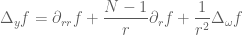
where  is the Laplace-Beltrami operator on the sphere. In particular, if f is a radial or spherically symmetric function (so by abuse of notation we write
  ), we have
 . (8)
. (8)
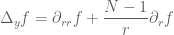
Now if we look at the high-dimensional limit  (noting that f, being radial, is well defined in every dimension), we see that the first order term
  dominates, despite the fact that
  is a second order operator. To clarify this domination (and to bring into view the operator
  appearing in (6)), let us make the change of variables
 (9)
(9)
(thus  is the average of the squared coordinates
  ). A quick application of the chain rule then yields
 (10)
(10)
(one can also see this by writing  and applying the Laplacian operator directly). If we restrict attention to the region of
  where all the coordinates
  are O(1), so
  and
and  , and fix
  while letting N go off to infinity, we thus see that converges to
  (with errors that are
  ).
).
Returning back to our ancient solution to the heat equation (6), it is now clear how to express this solution as a high-dimensional nearly harmonic function: if we define the high-dimensional lift  of u to the N+d-dimensional Euclidean space
  for some large N by using the change of variables (9), i.e.
 (11)
(11)
then we see from (10) and (6) that  is nearly harmonic as claimed; indeed we have
 (12)
(12)
in the region  , which implies as before that
 . (13)
Remark 3. Writing y in polar coordinates as  , the metric
  on
on  can be expressed as
 (14)
(14)
where  is the metric on the sphere
  of constant curvature
  . This expression is essentially the first equation in Section 6 of Perelman’s paper in the Euclidean case. Perelman works exclusively in polar coordinates, but I have found that the Cartesian coordinate approach can be more illuminating at times.
Remark 4. The formula (9) seems closely related to Itō’s formula  from stochastic calculus, combined perhaps with the central limit theorem, though I was not able to make this connection absolutely precise. Note that for reasons of duality, stochastic calculus tends to involve the backwards heat equation rather than the forwards heat equation (see e.g. the Black-Scholes formula), which seems to explain why the minus sign in (9) is not present in Itō’s formula.
To illustrate how this correspondence could be used, let us heuristically derive the classical formula
 (15)
(15)
for solutions to the heat equation (6) from the classical mean value principle
 (16)
(16)
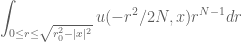
for harmonic functions . Actually, it will be slightly simpler to use the mean value principle for balls rather than spheres,
 , (17)
though in high dimensions there is actually very little difference between balls and spheres (the bulk of the volume of a high-dimensional ball is concentrated near its boundary, which is a sphere).
Let  and be as in (6) and (11). From (12) we see that is almost harmonic; let us be non-rigorous and pretend that is close enough to harmonic that the formula (17) remains accurate for this function. We write the volume of the ball
  as
as  for some constant
  . As for the integrand in (17), we use polar coordinates ,
  and rewrite (17) as
 (18)
(18)
for some other constant  . In view of (9), it is natural to write
  for some
  , and in view of (13) it is natural to work in the regime in which
  , and
, and  . Because
  is so rapidly increasing when N is large, the bulk of the inner integral is concentrated at its endpoint (cf. our previous remark about high-dimensional balls concentrating near their boundary), and so we expect
 . (19)
Since is so much larger than |x| in our regime of interest, we can heuristically approximate  by
by  . Also, by Taylor approximation we have
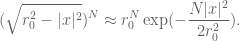 (20)
(20)
Putting all this together, and substituting  , we heuristically conclude
 (21)
(21)
for some other constant  . Taking limits as we heuristically obtain (15) up to a constant.
Exercise 4. Work through the calculations more carefully (but still heuristically), using Stirling’s approximation to the Gamma function, together with the classical formulae for the volume of balls and spheres, to verify that one does indeed get the right constant of  in (15) at the end of the day (as one must).
Now let us perform a variant of the above computations which is more closely related to the monotonicity of Perelman’s reduced volume. The Euclidean space is of course Ricci-flat, and so from Corollary 1 we know that the Bishop-Gromov reduced volume
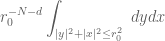 (22)
(22)
is non-decreasing in (and thus non-decreasing in  ). (Of course, being Euclidean, (22) is equal to a constant ; but let us ignore this fact (which we have already used in our heuristic derivation of (15)) for now.) Repeating all the above computations (but with u and replaced by 1) we thus heuristically conclude that the quantity
 (23)
(23)
is also non-decreasing in . (Indeed, this quantity is equal to  for all .) The quantity (23) is precisely the Perelman reduced volume of Euclidean space (which we view as a trivial example of an ancient Ricci flow) at the spacetime origin (0,0) and backwards time parameter .
— From Ricci flow to Ricci flat manifolds —
We have seen how ancient solutions to the heat equation on a Euclidean spacetime can be viewed as (approximately) harmonic functions on an “infinitely high dimensional” Euclidean space. Now we would like to analogously view ancient solutions to a heat equation on a flow of Riemannian manifolds as harmonic functions on an “infinitely high dimensional” Riemannian manifold, and similarly to view ancient Ricci flows as infinite dimensional infinitely high dimensional Ricci-flat manifolds.
Let’s begin with the former task. Starting with an ancient flow of d-dimensional Riemannian metrics for ![t \in (-\infty,0]](https://s0.wp.com/latex.php?latex=t+%5Cin+%28-%5Cinfty%2C0%5D&bg=ffffff&fg=545454&s=0&c=20201002) (which we will not assume to be a Ricci flow just yet) and a large integer N, we can consider the N+d-dimesional manifold
(which we will not assume to be a Ricci flow just yet) and a large integer N, we can consider the N+d-dimesional manifold  . As a first attempt to mimic the situation in the Euclidean case, it is natural to endow
  with the Riemannian metric
  given by the formula
 (24)
(24)
where t is given by the formula (9). In terms of local coordinates, if we use the indices a,b,c to denote the d indices for the x variable and i,j,k to denote the N indices for the y variable, we have
 (25)
(25)
where  is the Kronecker delta. From this we see that the volume measure
  on is given by
 (26)
(26)
and the Dirichlet form

 (27)
(27)

for this Riemannian manifold is given by
 , (28)
where  is the gradient of u in the x variable using the metric g(t). We can then integrate by parts to compute the Laplacian
  . Recalling that
  varies in t by the formula
 (29)
(29)
(equation (19) from Lecture 1) and using (9) and the chain rule, we see that
 (30)
(30)
where  is the Laplace-Beltrami operator in the x variable using the metric g(t). If we specialise to radial functions
 (31)
(31)
and use (10) and the chain rule, we can rewrite (29) as
 (32)
(32)
Thus we see that if u solves the heat equation  , then its lift
  is approximately harmonic in the sense that
  in the region where
  and x is confined to a compact region of space.
Remark 5. The  term in (32) is somewhat annoying; we will later tweak the metric (24) in order to remove it (at the cost of other, more acceptable, terms).
Now let us see whether Ricci flows  lift to approximately Ricci-flat manifolds . We begin by computing the Christoffel symbols
  in local coordinates, where
  refer to the N+d combined indices coming from the indices a on M and the indices i on . We recall the standard formula
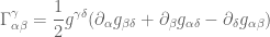 (33)
(33)
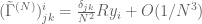
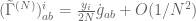
for the Christoffel symbols of a general Riemannian manifold in local coordinates. Specialising to the metric (25), some computation reveals that


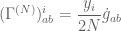 (34)
(34)

 .
.
Now the Ricci curvature  can be computed from the Christoffel symbols by the standard formula
 . (35)
If we apply this formula we obtain (after some computation)
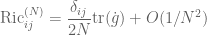
 (36)
(36)
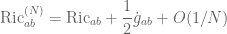 .
.
We thus see that if the original flow obeys the Ricci flow equation  , then the lifted manifold
  is nearly Ricci flat in the sense that all components of the Ricci curvature tensor are O(1/N) (in the region
  ). In fact the above estimates show that the Ricci curvature tensor is also O(1/N) in the operator norm sense and
  in the Hilbert-Schmidt (or Frobenius) sense.
It turns out that this approximation is not quite good enough for applications to Ricci flow, mainly because the 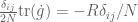 term in (36) gives a significant contribution to the trace of the Ricci tensor
  (i.e. the scalar curvature
  ), even in the limit . It turns out however that one can eliminate this problem by adding a correction term to the metric (24) involving the scalar curvature. More precisely, given an ancient Ricci flow , define the modified metric
  by the formula
 (37)
(37)
where of course  is the derivative of the radial variable r, and R(t,x) is the scalar curvature of g(t) at x. In coordinates, we have
 . (38)
Exercise 5. Let be a smooth ancient Ricci flow on ![(-\infty,0]](https://s0.wp.com/latex.php?latex=%28-%5Cinfty%2C0%5D&bg=ffffff&fg=545454&s=0&c=20201002) , and let be defined by (37). Show that in the region where
, and let be defined by (37). Show that in the region where  (so ) and x ranges in a compact set, the Christoffel symbols
  take the form

 (39)
(39)

 .
.
and the Ricci curvature  takes the form
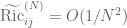
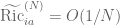 (40)
(40)
 .
.
In particular,  has norm in the trace (i.e. nuclear) norm (and hence in the Hilbert-Schmidt/Frobenius and operator norms).
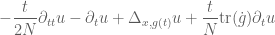
Exercise 6. Let the assumptions and notation be as in Exercise 5, let ![u: (-\infty,0] \times M \to {\Bbb R}](https://s0.wp.com/latex.php?latex=u%3A+%28-%5Cinfty%2C0%5D+%5Ctimes+M+%5Cto+%7B%5CBbb+R%7D&bg=ffffff&fg=545454&s=0&c=20201002) be a smooth function, and let be as in (31). Show that the Laplacian
be a smooth function, and let be as in (31). Show that the Laplacian  associated to obeys a similar formula to (32), but with the
  term replaced by terms which are
  when t, x are bounded.
— Perelman’s reduced length and reduced volume —
In the previous discussion, we have converted a Ricci flow to a Riemannian manifold  of much higher dimension which is almost Ricci flat. Let us adopt the heuristic that this latter manifold is sufficiently close to being Ricci flat that the Bishop-Gromov inequality (Corollary 1) holds (at least in the asymptotic limit ), thus the Bishop-Gromov reduced volume
  should heuristically be non-increasing in , where we fix a spatial origin
  .
.
In order to exploit the above heuristic, we first need to understand the distance function on  . Let
. Let  be a point in
  , and consider a length-minimising geodesic
 ![\gamma^{(N)}: [0,\tau_1] \to \tilde M](https://s0.wp.com/latex.php?latex=%5Cgamma%5E%7B%28N%29%7D%3A+%5B0%2C%5Ctau_1%5D+%5Cto+%5Ctilde+M&bg=ffffff&fg=545454&s=0&c=20201002) from
from  to
to  , where we have normalised the length
  of the parameter interval by the formula
  .
.
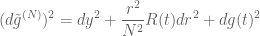
Observe that the metric (37) can be rewritten in polar coordinates (after substituting  ) as
) as
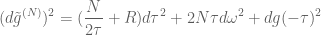 (41)
(41)
(which is essentially the first formula in Section 6 of Perelman’s paper). Note that the angular variable  only influences the second term in this metric and not the other two. Because of this, one sees that the geodesic
  must keep constant in order to be length-minimising (i.e.
  for the duration of the geodesic). Turning next to the variable, we then see that for N large enough, the geodesic should increase continuously from 0 to (as the
  term in (41) will severely penalise any backtracking. After a reparameterisation we may in fact assume that increases at constant speed, thus we have
 (42)
(42)
for some path ![\gamma: [0,\tau_1] \to M](https://s0.wp.com/latex.php?latex=%5Cgamma%3A+%5B0%2C%5Ctau_1%5D+%5Cto+M&bg=ffffff&fg=545454&s=0&c=20201002) from
from  to
to  . Using (41), the length of this geodesic is
 (43)
(43)
which by Taylor expansion is equal to
 (44)
(44)
where the  -length of
  is defined as
 (45)
(45)
Note that this quantity is independent of N. Thus, heuristically, geodesics in  from to
  should (approximately) minimise the -length. If we define
  to be the infimum of
  over all paths from to , we thus obtain the heuristic approximation
 . (46)
Exercise 7. When M is the Euclidean space (with the trivial Ricci flow, of course), show that  , and the minimiser is given by
  .
.
From (46) we see that the ball in of radius  centred at (where, as always, we are in the regime
  , so ) should heuristically take the form
 . (47)
If we make the plausible assumption that  varies smoothly in , then (47) is heuristically close (when N is large) to
 (48)
(48)
or equivalently
 . (49)
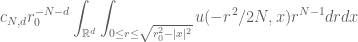
Now, the volume measure of (37) is of the form  , and so the volume of (49) is approximately
 . (50)
(Note there is a slight abuse of notation since  depends on
  , but it will soon be clear that this abuse is harmless.) When N is large, the inner integral is dominated by its right endpoint as before, and so (50) is approximately
 . (51)
We can Taylor expand this to be approximately
 (52)
(52)
where the Perelman reduced length  is defined as
 (53)
(53)
Example 1. Continuing the Euclidean example of Exercise 7, we have  , which is the familiar exponent in the fundamental solution (15). This is, of course, not a coincidence.
From (52) we thus heuristically conclude that the Bishop-Gromov reduced volume of at and at radius  is approximately equal to a constant multiple of
  , where the Perelman reduced volume is defined as
 . (54)
Example 2. Again continuing the Euclidean example, the reduced volume in Euclidean space (with the trivial Ricci flow) is always .
Formally applying Corollary 1, we are thus led to
Conjecture 1. (Monotonicity of Perelman reduced volume) Let be a Ricci flow on ![{}[-T,0]](https://s0.wp.com/latex.php?latex=%7B%7D%5B-T%2C0%5D&bg=ffffff&fg=545454&s=0&c=20201002) , and let
, and let  . Then the quantity for
  is monotone non-increasing in .
Remark 6. Note here we are not taking the Ricci flow to be ancient; this would correspond to the manifold being replaced by an incomplete manifold, of radius about  . However, because of the restriction
  , the above heuristic arguments never “encounter” the lack of completeness, and so it is reasonable to expect that the conjecture will continue to hold in the non-ancient case. This is of course an essential point for our applications, since the Ricci flows we study are not assumed to be ancient.
Remark 7. At an crude heuristic level, the Perelman reduced volume is roughly like  (since, in view of Exercise 7, we expect
  to behave like
  , especially in regions of bounded normalised curvature, where we are deliberately vague about exactly what metric we using to define d). This heuristic suggests that Conjecture 1 should be able to establish the non-collapsing result we want (Theorem 2 from Lecture 7). This will be made more rigorous in subsequent lectures. For now, we observe that the Perelman reduced length and reduced volume are dimensionless (just as the Bishop-Gromov reduced volume is), which as discussed in Lecture 7 is basically a necessary condition in order for this quantity to force non-collapsing of the geometry.
As far as I am aware, there is no rigorous proof of Conjecture 1 that follows the above high-dimensional comparison geometry heuristic argument. Nevertheless, it is possible to prove Conjecture 1 by other means, and in particular by developing parabolic analogues of all the comparison geometry machinery that is used to prove the Bishop-Gromov inequality (and in particular, developing a theory of -geodesics analogous to the “elliptic” theory of geodesics on a Riemannian manifold. This will be the focus of the next few lectures.
Remark 8. It seems of interest to try to make the above arguments more rigorous, and to expand the dictionary between elliptic and parabolic equations. I do not know however of much literature in this direction, apart from Section 6 of Perelman’s original paper (see also Section 3.1 of Cao-Zhu), in which a few other parabolic notions (e.g. the backwards heat equation, or the modified Ricci flow from the previous lecture) are reinterpreted as high-dimensional elliptic notions. See however the work of Chow and Chu (see also this sequel paper), which views parabolic theory as a degenerate version of elliptic theory; Perelman’s viewpoint can be interpreted as a regularisation of Chow-Chu’s viewpoint.


24 comments
Comments feed for this article
27 April, 2008 at 11:55 pm
Pedro Lauridsen Ribeiro
Dear Prof. Tao,
I don’t know if it’s related, but the infinite-dimensional limit dealt with in this , where
  is the number of steps
lecture (as well as parabolic theory being an infinite-dimensional limit of elliptic theory) does ring me a bell about the derivation of the heat equation from Brownian motion. The infinite-dimensional Riemannian manifold in question
would be the space of Brownian paths in the original Riemannian manifold, up
to some time rescaling – indeed, recall that the time variable has the
dimension of
in the random walk. Moreover, we also know that the heat kernel is the
(infinite-dimensional) Fourier transform of a Gaussian measure in the space
of random fields which are the continuum limit of Brownian paths, by the Bochner-Minlos theorem. It seems, judging, for example, by the work
of Grigor’yan and others on the heat kernel in complete Riemannian manifolds, that much of this derivation can be performed for more general Riemannian manifolds, under assumptions on the geometry which are similar to those underlying the Bishop-Gromov formula.
2 May, 2008 at 11:32 am
Anon
Hi,
I was wondering if there was a link that categorized all the Ricci Flow/Poincare Conjecture articles into one webpage? I’m having trouble finding the first lecture and working my way to the present article.
Thanks.
2 May, 2008 at 12:47 pm
Terence Tao
Dear Anon,
You can try
https://terrytao.wordpress.com/category/teaching/285g-poincare-conjecture/
(For some reason, my articles are not being picked up by the global wordpress tag system, so the links just below the article titles are not working properly, but presumably this will sort itself out at some point.)
Dear Pedro: Thanks for the interesting comments; what you say sounds broadly consistent with my own speculations on the role of Brownian motion in this limit (see Remark 4 above). It would be nice to have a precise connection, though, even in the Euclidean case.
9 May, 2008 at 7:40 am
285G, Lecture 10: Variation of L-geodesics, and monotonicity of Perelman reduced volume « What’s new
[…] a heuristic derivation of the monotonicity of Perelman reduced volume (Conjecture 1 from the previous lecture), we now turn to a rigorous proof. Whereas in the previous lecture we […]
19 May, 2008 at 10:00 am
285G, Lecture 11: κ-noncollapsing via Perelman reduced volume « What’s new
[…] reduced volume in the previous lecture (after first heuristically justifying this monotonicity in Lecture 9), we now show how this can be used to establish -noncollapsing of Ricci flows, thus giving a second […]
19 May, 2008 at 10:13 am
285G, Lecture 13: Li-Yau-Hamilton Harnack inequalities and κ-solutions « What’s new
[…] one by Chow and Chu using a metric closely related to the high-dimensional metrics considered in Lecture 9, but all of the proofs I know of require a significant amount of […]
21 May, 2008 at 1:04 pm
285G, Lecture 14: Stationary points of Perelman entropy or reduced volume are gradient shrinking solitons « What’s new
[…] we first consider the simpler model case of the Bishop-Gromov reduced volume (Corollary 1 of Lecture 9). An inspection of the proof of that result reveals that the key point was to establish the […]
27 May, 2008 at 6:06 pm
285G, Lecture 15: Geometric limits of Ricci flows, and asymptotic gradient shrinking solitons « What’s new
[…] large n. Also, from the curvature bounds and Bishop-Gromov comparison geometry (Lemma 1 from Lecture 9) we know that the volume of is uniformly bounded from above for sufficiently large […]
30 May, 2008 at 10:25 pm
285G, Lecture 16: Classification of asymptotic gradient shrinking solitons « What’s new
[…] geometry of constant curvature K, much as in the discussion of the Bishop-Gromov inequality in Lecture 9. See Petersen’s book for […]
2 June, 2008 at 1:29 am
Pedro Lauridsen Ribeiro
There’s an issue that puzzles me about the Bishop-Gromov volume comparison theorem, especially in the case of non-negative Ricci curvature.
If we look at balls of (small) radius
  inside geodesically convex charts centered, say, at
  , we can think of the Radon-Nikodym derivative of the measure induced by the Riemannian metric w.r.t. the one induced by the Euclidean metric in the chart (which is just the Lebesgue measure) at
  as the limit of (a constant which depends only on the dimension times) the Bishop-Gromov reduced volume of
  as
as  . The Bishop-Gromov inequality seems to imply that the Radon-Nikodym derivative at
  equals 1. So far, nothing strange.
What seems puzzling to me is that, if is the usual Riemannian
 in
in  by first defining
  and then extending it to all Borel sets by means of Caratheodory’s construction of outer measures (the latter can be modified so as to guarantee that
  for all Borel sets
  such that
  ), then not only will
  match Lebesgue measure in Riemannian normal charts for small geodesically convex balls, but, by the reasoning in the previous paragraph, we will have that
  (almost) everywhere, however these two measures are not equal in general! Am I missing or screwing up something in my reasoning above?
measure and we define a new measure
2 June, 2008 at 4:28 pm
Terence Tao
Dear Pedro,
Caratheodory’s construction requires the volumes that one assigns to balls to be compatible: if for instance one ball is the countable disjoint union of many other balls, then the volume assigned to the former ball must be the sum of the volume assigned to the latter. The balls you propose will not have this property (think about what happens, say, on the round sphere ).
).
2 June, 2008 at 11:26 pm
Pedro Lauridsen Ribeiro
So, the problem is what happens to _large_ (i.e. non geodesically convex) balls, I suppose? Because for small balls in geodesically convex neighbourhoods, as defined in my last post is just Lebesgue measure in Riemann normal coordinates, and for those countable disjoint coverings by smaller balls should give the right result.
3 June, 2008 at 8:14 am
Terence Tao
Dear Pedro,
The measure formed from Lebesgue measure on normal coordinates from one point x are not the same as the measure formed by Lebesgue measure on normal coordinates from another point y, unless the manifold happens to be flat. Thus, for instance, you can have B(x,r) have Euclidean volume for all r (up to the injectivity radius, at least), or B(y,r) have Euclidean volume for all r, but in general you can’t have both simultaneously with a single measure, due to the presence of curvature. For instance, in hyperbolic space one can pack many more small balls of radius r disjointly into a large ball of radius R than in Euclidean space (indeed, in hyperbolic space the packing number grows exponentially in R for fixed r). Here the problem is not failure of injectivity (normal coordinates are global here), but the constant presence of negative curvature.
3 June, 2008 at 10:44 am
Pedro Lauridsen Ribeiro
Now I see my mistake… :-p Thanks a lot!
10 July, 2008 at 12:02 pm
ky
If somebody could please explain in more detail the derivation behind the five formulas in (34) involving Christoffel symbols and the three formulas in (36) involving Ric, it would be really great.
Thanks you.
10 July, 2008 at 2:40 pm
JC
ky:
For (34), simply use the expressions for the metric in (25) into the formula (33), and calculate, e.g. the first equation:
Now implies that the last term vanishes (since it’s a constant). The second and third terms you can break into the
  type terms (when the index
  ), which are zero from (25), and also
  terms (when the index
  ) which are
  and hence zero after differentiation with respect to
  …
…
For (36), just use the equations derived in (34) in evaluating the components of (35) in a similar way. Is this what you meant?
12 July, 2008 at 10:27 am
ky
JC:
Thank you so much. As a student, while I took baby Riemannian Geometry course, I never understood the Christoffel symbol fully. With you help, I got the first 2 of (34). But when it comes to the last 3 of (34) and (36) I am still struggling; e.g. the N on the denominator and y_i on the numerator. If you could get me started with those the way you did for the first one in (34), I would appreciate it.
27 August, 2008 at 9:14 am
Tricks Wiki article: The tensor product trick « What’s new
[…] Example 8. (Monotonicity of Perelman’s reduced volume) One of the key ingredients of Perelman’s proof of the Poincaré conjecture is a monotonicity formula for Ricci flows, that establishes that a certain geometric quantity, now known as the Perelman reduced volume, increases as time goes to negative infinity. Perelman gave both a rigorous proof and a heuristic proof of this formula. The heuristic proof is much shorter, and proceeds by first (formally) applying the Bishop-Gromov inequality for Ricci flat metrics (which shows that another geometric quantity – the Bishop-Gromov reduced volume, increases as the radius goes to infinity) not to the Ricci flow itself, but to a high-dimensional version of this Ricci flow formed by adjoining an M-dimensional sphere to the flow in a certain way, and then taking (formal) limits as . This is not precisely the tensor power trick, but is certainly in a similar spirit. For further discussion see “285G Lecture 9: Comparison geometry, the high-dimensional limit, and Perelman’s reduced volume.” […]
29 March, 2009 at 4:12 am
Mikhail Gromov wins 2009 Abel prize « What’s new
[…] geometry (which (together with its parabolic variant, the monotonicity of Perelman reduced volume) plays an important role in Perelman’s proof of the Poincaré conjecture), the concept of Gromov-Hausdorff convergence […]
13 November, 2011 at 5:21 pm
254A, Notes 9: Applications of the structural theory of approximate groups « What’s new
[…] of Ricci curvature, which would be beyond the scope of these notes); but see for instance this previous blog post of mine for a proof. This inequality is consistent with the geometric intuition that an increase in […]
5 September, 2013 at 9:23 pm
Notes on simple groups of Lie type | What's new
[…] and sectional curvatures uniformly bounded from below. Applying Myers’ theorem (discussed in this previous blog post), we conclude that any cover of is necessarily compact also; this implies that the fundamental […]
14 February, 2022 at 4:46 pm
Yifan
I think in formula (10), we should get -2t/N \partial_{tt} f-\partial_t f and also in formula (12) we should have r^2/N^2 \partial_{tt} u-\partial_t u+\Delta_x u
[Corrected, thanks – T.]
14 February, 2022 at 5:22 pm
Yifan
Also in formula (20) RHS should be r_0^N exp(-N|x|^2/(2r_0^2))
[Corrected, thanks – T.]
19 February, 2022 at 7:49 pm
Yifan
Again some typos: in formula (49) (50) (51), it should be
[Corrected, thanks – T.]