
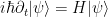
is the fundamental equation of motion for (non-relativistic) quantum mechanics, modeling both one-particle systems and 


I recently attended a talk by Natasa Pavlovic on the rigorous derivation of this type of limiting behaviour, which was initiated by the pioneering work of Hepp and Spohn, and has now attracted a vast recent literature. The rigorous details here are rather sophisticated; but the heuristic explanation of the phenomenon is fairly simple, and actually rather pretty in my opinion, involving the foundational quantum mechanics of
This discussion will be purely formal, in the sense that (important) analytic issues such as differentiability, existence and uniqueness, etc. will be largely ignored.
— 1. A quick review of classical mechanics —
The phenomena discussed here are purely quantum mechanical in nature, but to motivate the quantum mechanical discussion, it is helpful to first quickly review the more familiar (and more conceptually intuitive) classical situation.
Classical mechanics can be formulated in a number of essentially equivalent ways: Newtonian, Hamiltonian, and Lagrangian. The formalism of Hamiltonian mechanics for a given physical system can be summarised briefly as follows:
- The physical system has a phase space
of states
(which is often parameterised by position variables
and momentum variables
). Mathematically, it has the structure of a symplectic manifold, with some symplectic form
(which would be
if one had position and momentum coordinates available).
- The complete state of the system at any given time
is given (in the case of pure states) by a point
in the phase space
- Every physical observable (e.g., energy, momentum, position, etc.)
is associated to a function (also called
). If one measures the observable
.
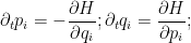
- There is a special observable, the Hamiltonian
, which governs the evolution of the state
, these equations are given by the formulae
more abstractly, just from the symplectic form
where
is the symplectic gradient of
.

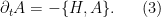
Hamilton’s equation of motion can also be expressed in a dual form in terms of observables

for any observable 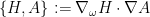
In the above formalism, we are assuming that the system is in a pure state at each time 


The equation of motion of a mixed state 

using the same vector field 
Pure states can be viewed as the special case of mixed states in which the probability distribution 

Suppose one had a 


then the equations of motion for the first and second particles would be completely decoupled, with no interactions between the two particles. However, in practice, the joint Hamiltonian contains coupling terms between 
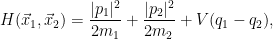
where 


In a similar spirit, a mixed joint state is a joint probability distribution 

(for the first particle) or
(for the second particle). Similarly for 
the distribution of the first two particles is given by
and so forth.
A typical Hamiltonian in this case may take the form
which is a combination of single-particle Hamiltonians 


Now imagine a system of 


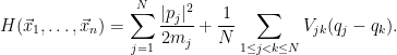
A typical example of a symmetric Hamiltonian is

where 


where 


An important example of a symmetric mixed state is a factored state

where 
— 2. A quick review of quantum mechanics —
Now we turn to quantum mechanics. This theory is fundamentally rather different in nature than classical mechanics (in the sense that the basic objects, such as states and observables, are a different type of mathematical object than in the classical case), but shares many features in common also, particularly those relating to the Hamiltonian and other observables. (This relationship is made more precise via the correspondence principle, and more precise still using semi-classical analysis.)
The formalism of quantum mechanics for a given physical system can be summarised briefly as follows:
- The physical system has a phase space
of states
- The complete state of the system at any given time
in the phase space
- Every physical observable
. (The full distribution of
- There is a special observable, the Hamiltonian
, which governs the evolution of the state

Schrödinger’s equation of motion can also be expressed in a dual form in terms of observables
![\displaystyle \partial_t \langle \psi | A | \psi \rangle = \frac{i}{\hbar} \langle \psi | [ H, A ] | \psi \rangle](https://s0.wp.com/latex.php?latex=%5Cdisplaystyle++%5Cpartial_t+%5Clangle+%5Cpsi+%7C+A+%7C+%5Cpsi+%5Crangle+%3D+%5Cfrac%7Bi%7D%7B%5Chbar%7D+%5Clangle+%5Cpsi+%7C+%5B+H%2C+A+%5D+%7C+%5Cpsi+%5Crangle&bg=ffffff&fg=000000&s=0&c=20201002)
![\displaystyle \partial_t A = \frac{i}{\hbar} [ H, A ] \ \ \ \ \ (6)](https://s0.wp.com/latex.php?latex=%5Cdisplaystyle++%5Cpartial_t+A+%3D+%5Cfrac%7Bi%7D%7B%5Chbar%7D+%5B+H%2C+A+%5D+%5C+%5C+%5C+%5C+%5C+%286%29&bg=ffffff&fg=000000&s=0&c=20201002)
where ![{[,]}](https://s0.wp.com/latex.php?latex=%7B%5B%2C%5D%7D&bg=ffffff&fg=000000&s=0&c=20201002)
The states 


![\displaystyle \partial_t \rho = \frac{i}{\hbar} [H,\rho]. \ \ \ \ \ (7)](https://s0.wp.com/latex.php?latex=%5Cdisplaystyle++%5Cpartial_t+%5Crho+%3D+%5Cfrac%7Bi%7D%7B%5Chbar%7D+%5BH%2C%5Crho%5D.+%5C+%5C+%5C+%5C+%5C+%287%29&bg=ffffff&fg=000000&s=0&c=20201002)
One can view pure states as the special case of mixed states which are rank one projections,

Morally speaking, the space of mixed states is the convex hull of the space of pure states (just as in the classical case), though things are a little trickier than this when the phase space
Pure states suffer from a phase ambiguity: a phase rotation 

In a single particle system, modeling a (scalar) quantum particle in a 


as 


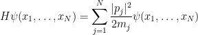
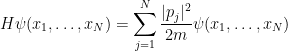
A typical Hamiltonian in this setting is given by the operator

where 


Now suppose one has an 
and a mixed state is a Hermitian positive semi-definite function 

with a pure state

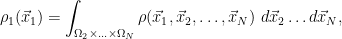
In classical mechanics, the state of a single particle was the marginal distribution of the joint state. In quantum mechanics, the state of a single particle is instead obtained as the partial trace of the joint state. For instance, the state of the first particle is given as

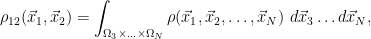
the state of the first two particles is given as


and so forth. (These formulae can be justified by considering observables of the joint state that only affect, say, the first two position coordinates 
A typical Hamiltonian in this setting is given by the operator

where we normalise just as in the classical case, and 
An interesting feature of quantum mechanics – not present in the classical world – is that even if the
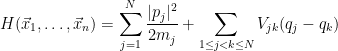
Now consider a system of

for some even potential

for some 
— 3. NLS —
Suppose we have a Bose-Einstein condensate given by a (symmetric) mixed state

evolving according to the equation of motion (7) using the Hamiltonian (8). One can take a partial trace of the equation of motion (7) to obtain an equation for the state 

![\displaystyle + \frac{1}{N} \sum_{j=2}^N \int_{{\mathbb R}^d} \frac{1}{r^d} [ V( \frac{x_1 - x_j}{r} ) - V( \frac{x'_1 -x_j}{r} ) ] \rho_{1j}(t,x_1,x_j; x'_1,x_j)\ dx_j](https://s0.wp.com/latex.php?latex=%5Cdisplaystyle++%2B+%5Cfrac%7B1%7D%7BN%7D+%5Csum_%7Bj%3D2%7D%5EN+%5Cint_%7B%7B%5Cmathbb+R%7D%5Ed%7D+%5Cfrac%7B1%7D%7Br%5Ed%7D+%5B+V%28+%5Cfrac%7Bx_1+-+x_j%7D%7Br%7D+%29+-+V%28+%5Cfrac%7Bx%27_1+-x_j%7D%7Br%7D+%29+%5D+%5Crho_%7B1j%7D%28t%2Cx_1%2Cx_j%3B+x%27_1%2Cx_j%29%5C+dx_j&bg=ffffff&fg=000000&s=0&c=20201002)
where 


![\displaystyle + \frac{N-1}{N} \int_{{\mathbb R}^d} \frac{1}{r^d} [ V( \frac{x_1 - x_2}{r} ) - V( \frac{x'_1 -x_2}{r} ) ] \rho_{12}(t,x_1,x_2; x'_1,x_2)\ dx_2.](https://s0.wp.com/latex.php?latex=%5Cdisplaystyle++%2B+%5Cfrac%7BN-1%7D%7BN%7D+%5Cint_%7B%7B%5Cmathbb+R%7D%5Ed%7D+%5Cfrac%7B1%7D%7Br%5Ed%7D+%5B+V%28+%5Cfrac%7Bx_1+-+x_2%7D%7Br%7D+%29+-+V%28+%5Cfrac%7Bx%27_1+-x_2%7D%7Br%7D+%29+%5D+%5Crho_%7B12%7D%28t%2Cx_1%2Cx_2%3B+x%27_1%2Cx_2%29%5C+dx_2.&bg=ffffff&fg=000000&s=0&c=20201002)
This does not completely describe the dynamics of 

Let us now formally take two limits in the above equation, sending the number of particles 


![\displaystyle + \lambda (\rho_{12}(t,x_1,x_1;x'_1,x_1) - \rho_{12}(t,x_1,x'_1;x'_1,x'_1)) ].](https://s0.wp.com/latex.php?latex=%5Cdisplaystyle++%2B+%5Clambda+%28%5Crho_%7B12%7D%28t%2Cx_1%2Cx_1%3Bx%27_1%2Cx_1%29+-+%5Crho_%7B12%7D%28t%2Cx_1%2Cx%27_1%3Bx%27_1%2Cx%27_1%29%29+%5D.&bg=ffffff&fg=000000&s=0&c=20201002)
One can perform a similar formal limiting procedure for the other equations in the BBGKY hierarchy, obtaining a system of equations known as the Gross-Pitaevskii hierarchy.
We next make an important simplifying assumption, which is that in the limit

One can view this as a mean field approximation, modeling the interaction of one particle 
Making this assumption, the previous equation simplifies to
![\displaystyle + \lambda (\rho_1(t,x_1;x_1) - \rho_1(t,x'_1;x'_1))] \rho_1(t,x_1;x'_1).](https://s0.wp.com/latex.php?latex=%5Cdisplaystyle+%2B+%5Clambda+%28%5Crho_1%28t%2Cx_1%3Bx_1%29+-+%5Crho_1%28t%2Cx%27_1%3Bx%27_1%29%29%5D+%5Crho_1%28t%2Cx_1%3Bx%27_1%29.&bg=ffffff&fg=000000&s=0&c=20201002)
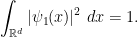
If we assume furthermore that

then (up to the phase ambiguity mentioned earlier), 
![\displaystyle \partial_t \psi(t,x) = \frac{i}{\hbar} [ (\frac{|p|^2}{2m} + \lambda |\psi(t,x)|^2 ] \psi(t,x)](https://s0.wp.com/latex.php?latex=%5Cdisplaystyle++%5Cpartial_t+%5Cpsi%28t%2Cx%29+%3D+%5Cfrac%7Bi%7D%7B%5Chbar%7D+%5B+%28%5Cfrac%7B%7Cp%7C%5E2%7D%7B2m%7D+%2B+%5Clambda+%7C%5Cpsi%28t%2Cx%29%7C%5E2+%5D+%5Cpsi%28t%2Cx%29&bg=ffffff&fg=000000&s=0&c=20201002)
which (up to some factors of 
An alternate derivation of (1), using a slight variant of the above mean field approximation, comes from studying the Hamiltonian (8). Let us make the (very strong) assumption that at some fixed time

where 
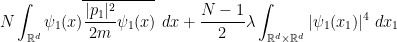
(This is an unrealistically strong version of the mean field approximation. In practice, one only needs the two-particle partial traces to be completely factored for the discussion below.) The expected value of the Hamiltonian,

can then be simplified as


Again sending 
which in the limit
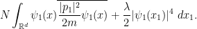
Up to some normalisations, this is the Hamiltonian for the NLS equation (1).
There has been much progress recently in making the above derivations precise, by Erdös-Schlein-Yau, Klainerman-Machedon, Kirkpatrick-Schlein-Staffilani, Chen-Pavlovic, and others. A key step is to show that the Gross-Pitaevskii hierarchy necessarily preserves the property of being a completely factored state. This requires a uniqueness theory for this hierarchy, which is surprisingly delicate, due to the fact that it is a system of infinitely many coupled equations over an unbounded number of variables.
[Update, Dec 8: Interestingly, the above heuristic derivation only works when the interaction scale 


14 comments
Comments feed for this article
26 November, 2009 at 10:25 pm
Anonymous
Professor Tao:
In the third paragraph, do you mean to say that the discussion will be purely informal?
26 November, 2009 at 11:39 pm
Anonymous
Mathematicians tend to use the word “formal” to describe an argument in which symbolic manipulations may not be justified rigorously. (You just cross your fingers and hope for the best.)
27 November, 2009 at 2:46 am
Mio
Dear Prof. Tao, looks like there’s a typo in (7), A should be H instead. Also, the ket above (6) is missing a \psi inside. Thanks for the post.
[Corrected, thanks – T.]
28 November, 2009 at 2:28 pm
M.S.
Really beautiful and clear, as your other post!
It made me enjoy my long train trip today, thanks.
I saw a typo immediately before the introduction of the interaction potential sum normalization, I think it should be:
If the momenta $p_j$ and masses $m_j$ are normalised to be of size
[Corrected, thanks – T.]
29 November, 2009 at 3:53 pm
CJ
Prof. Tao–There seems to be a missing equation in your definition of Hamilton’s equations on a sympletic manifold, right after “the equations of motion can be written as”.
29 November, 2009 at 3:58 pm
CJ
Prof. Tao–Actually, it looks like all the numbered equations are having difficulties being displayed. (At least I don’t see them running firefox on Ubuntu.)
[Hmm, a strange glitch – I think the equations are restored now. -T]
30 November, 2009 at 7:41 am
liuyao
minor typo: , the prime on x, not on
 , though the minus sign is immaterial when you square it, and is more of a convention.
Momentum is usually identified with
Great post, by the way!
[Corrected, thanks – T.]
1 December, 2009 at 1:40 am
A semana nos arXivs… « Ars Physica
[…] From Bose-Einstein condensates to the nonlinear Schrodinger equation […]
2 December, 2009 at 2:29 pm
John Sidles
Please let me echo the above comments in saying that this is a wonderfully interesting and enjoyable post!
I would like to offer three comments on how engineering students might read (and mis-read) this post, recornizing that increasing numbers of engineering students are seeking to upgrade their mathematical understanding.
None of the following remarks should be construed as being in any respect critical of Prof. Tao’s fine essay. Rather, they should be read as fan mail—-and as an expression of thanks—from the engineering community to the mathematical community.
One of Bjarne Stroustrup’s maxims is “Whenever something can be done in two ways, someone will be confused.” And when it comes to quantum mechanics—with its plethora of invariances and conventions–few people are more easily confused than literal-minded engineering students!
Engineering students can become confused in ways that might not occur to mathematicians, as follows:
(1) When discussing dynamical state-spaces endowed with a metric and/or symplectic structure, is it better to give equations in terms of vectors, or in terms of forms? Mathematicians are happy either way, but they tend to choose vector frameworks (as Tao’s essay does), perhaps for the reason that vectors are easier to sketch than forms.
However, if we have in mind (sooner or later) to pullback dynamical equations onto lower-dimension, noneuclidean manifolds (as engineers ubiquitously do), then it is convenient to express dynamical equations (and complex structures, etc.) in terms of forms rather than vectors … and it helps engineering students to be reminded that forms pullback naturally and vectors don’t.
This boils down to assuring students that symplectic gradients can be defined to map functions to vectors, or alternatively map functions to forms, with equal validity (given a symplectic and/or metric structure that establishes a natural isomorphism).
(2) On the arxiv server there is a (unpublished, but very clear) essay by Prof. Tao titled Perelman’s proof of the Poincare conjecture: a nonlinear PDE perspective (arXiv.org:math/0610903). In particular, footnote three of this article is in itself a short yet powerfully thought-provoking essay to the effect that “a PDE flow is in many ways ‘dumber’ than a combinatorial algorithm than a combinatorial algorithm” and yet “if the flow is sufficiently geometrical in nature then the flows acquire a number of deep and delicate additional properties”.
In quantum mechanics as in topology, there is steadily increasing use of flow/PDE algorithms in conjunction with combinatorical/algebraic algorithms; an essay on this general topic would be *very* welcome (IMHO) to many students/researchers in quantum mechanics (in engineering and otherwise).
(3) Quantum mechanics has a reputation for being mysterious, and in particular, there is a widespread impression that its basic postulates are inviolate. But as is often the case with no-go arguments, a loophole exists that Prof. Tao’s present essay illustrates beautifully.
That loophole is that (in Prof. Tao’s words) “despite [quantum dynamics] being a linear equation, solutions can be governed by a non-linear equation”. Thus we are free to invent nonlinear versions of quantum mechanics, without fear of experimental contradiction, provided that we can derive the nonlinear dynamics from linear quantum mechanics.
This principle applies broadly in quantum mechanics and many other physical theories; for example there is a recent article by Stephen Adler and Angelo Bassi titled Is Quantum Theory Exact? that can be read as an another example of this same general principle.
Here too an essay on “Mathematical methods for circumventing no-go arguments in physical theories” would be very interesting—and very stimulating too!—to many students.
That’s all! And thanks also, to everyone who contributes what is becoming (IMHO) the present-day “Golden Era of Mathematical Blogging”. :)
8 December, 2009 at 10:29 am
Bob Jerrard
nice post. just a few days ago I saw a talk by Laszlo Erdos on some of his work (with Schlein and Yau and others) on these problems, and he emphasized that the correct value of the coupling constant is not the total mass of the interaction potential
  , but rather is
  , where
  is the scattering length, defined as follows: consider a solution
  of the equation
  in
in  , such that
  at
at  . Then if the potential
  is sufficiently short-range, it is a fact that
  is asymptotic to
  for some
  (for example this is clear if
  is compactly supported), and the constant
  is defined to be the scattering length.
In order to see the scattering length appear in the Gross-Pitaevsky equation, one needs to modify the product state ansatz you have given above. The modified ansatz has the form
writing it for wave functions rather than density matrices, and so takes into account short-range correlations between particles. If I understand correctly, the definitions of and
and  imply that
and it is via this fact that the above modified ansatz gives rise to in the GP equation.
The justification of the limit thus requires establishing some information about short-range repulsive interactions between particles.
8 December, 2009 at 12:15 pm
Terence Tao
That’s a very interesting subtlety! I think it shows up for some ranges of r and N and not others, in particular if the range r of the potential is significantly longer than the mean spacing of the particles then the naive approximation should work, I think (this is for instance the case in the Chen-Pavlovic work, where the potential is rather long range and the nonlinear correction does not appear).
It is good to have examples of why one should not always trust naive limiting arguments, though…
8 December, 2009 at 6:44 pm
H.S.
Thank you for this wonderful post. I just have a couple of questions:
1) For classical interacting system, what is the “interesting limit” you mentioned in the post? Could you please explain more about that limit? For instance is there a nonlinear equation in the limit? The power law of r and N is kind of mysterious to me. What’s the value of the exponent there explicitly?
2) In quantum case, has the Mean field approximation that the two-particle mixed state can factorize in the limit been rigorously justified? [In classical case at positive temperature, there’re “propagation of chaos” type results, which can justify mean field approximation].
3) I feel like, usually, mean field approximation is valid only for long range interactions. But here we are concerned about short range interactions. Well, this is not actually a question, maybe my feeling is just incorrect.
Thank you again!
8 December, 2009 at 7:07 pm
Terence Tao
(1) I don’t have a formal derivation, but it seems to me that the limiting dynamics of the classical model should be governed by the one-particle advection equation but with an effective Hamiltonian containing a potential term proportional to the spatial density . There is undoubtedly a name for this type of nonlinear kinetic equation but it escapes me at the moment. This type of limit should obtain whenever r is much smaller than 1 but much larger than 1/N; for r=1/N I suppose one should have a correction in analogy with the quantum case as pointed out by Bob Jerrard above.
(2) As far as I am aware, most of the rigorous results require the initial state to already be factored or close to factored, and the conclusion is that this near-factored property is more or less preserved (with dynamics given by the effective equation). There are certainly efforts to generalise to broader classes of data, though.
(3) There is a parallel set of results for long-range interactions, in which the nonlinearity becomes nonlocal (of Hartree type, generally).
26 September, 2014 at 4:10 am
My great WordPress blog – Econlinks
[…] Tao makes a nice and concise exposition of some of the most beautiful parts at the intersection of Mathematics and Theoretical Physics (oh, nostalgia…), including quick reviews of classical and quantum […]