
In the foundations of modern probability, as laid out by Kolmogorov, the basic objects of study are constructed in the following order:
- Firstly, one selects a sample space
, whose elements
represent all the possible states that one’s stochastic system could be in.
- Then, one selects a
-algebra
of events
(modeled by subsets of
in a countably additive manner, so that the entire sample space has probability
.
- Finally, one builds (commutative) algebras of random variables
(such as complex-valued random variables, modeled by measurable functions from
), and (assuming suitable integrability or moment conditions) one can assign expectations
to each such random variable.
In measure theory, the underlying measure space
However, it is possible to take the abstraction process one step further, and view the algebra of random variables and their expectations as being the foundational concept, and ignoring both the presence of the original sample space, the algebra of events, or the probability measure.
There are two reasons for wanting to shed (or abstract away) these previously foundational structures. Firstly, it allows one to more easily take certain types of limits, such as the large 


Secondly, this abstract formalism allows one to generalise the classical, commutative theory of probability to the more general theory of non-commutative probability theory, which does not have a classical underlying sample space or event space, but is instead built upon a (possibly) non-commutative algebra of random variables (or “observables”) and their expectations (or “traces”). This more general formalism not only encompasses classical probability, but also spectral theory (with matrices or operators taking the role of random variables, and the trace taking the role of expectation), random matrix theory (which can be viewed as a natural blend of classical probability and spectral theory), and quantum mechanics (with physical observables taking the role of random variables, and their expected value on a given quantum state being the expectation). It is also part of a more general “non-commutative way of thinking” (of which non-commutative geometry is the most prominent example), in which a space is understood primarily in terms of the ring or algebra of functions (or function-like objects, such as sections of bundles) placed on top of that space, and then the space itself is largely abstracted away in order to allow the algebraic structures to become less commutative. In short, the idea is to make algebra the foundation of the theory, as opposed to other possible choices of foundations such as sets, measures, categories, etc..
[Note that this foundational preference is to some extent a metamathematical one rather than a mathematical one; in many cases it is possible to rewrite the theory in a mathematically equivalent form so that some other mathematical structure becomes designated as the foundational one, much as probability theory can be equivalently formulated as the measure theory of probability measures. However, this does not negate the fact that a different choice of foundations can lead to a different way of thinking about the subject, and thus to ask a different set of questions and to discover a different set of proofs and solutions. Thus it is often of value to understand multiple foundational perspectives at once, to get a truly stereoscopic view of the subject.]
It turns out that non-commutative probability can be modeled using operator algebras such as 
When one generalises the set of structures in one’s theory, for instance from the commutative setting to the non-commutative setting, the notion of what it means for a structure to be “universal”, “free”, or “independent” can change. The most familiar example of this comes from group theory. If one restricts attention to the category of abelian groups, then the “freest” object one can generate from two generators 


Similarly, when generalising classical probability theory to non-commutative probability theory, the notion of what it means for two or more random variables to be independent changes. In the classical (commutative) setting, two (bounded, real-valued) random variables 
whenever 


whenever 

The concept of free independence was introduced by Voiculescu, and its study is now known as the subject of free probability. We will not attempt a systematic survey of this subject here; for this, we refer the reader to the surveys of Speicher and of Biane. Instead, we shall just discuss a small number of topics in this area to give the flavour of the subject only.
The significance of free probability to random matrix theory lies in the fundamental observation that random matrices which are independent in the classical sense, also tend to be independent in the free probability sense, in the large
Much as free groups are in some sense “maximally non-commutative”, freely independent random variables are about as far from being commuting as possible. For instance, if 


Another important (and closely related) analogy is that while the distribution of sums of independent commutative random variables can be quickly computed via the characteristic function (i.e. the Fourier transform of the distribution), the distribution of sums of freely independent non-commutative random variables can be quickly computed using the Stieltjes transform instead (or with closely related objects, such as the 
As mentioned earlier, free probability is an excellent tool for computing various expressions of interest in random matrix theory, such as asymptotic values of normalised moments in the large 


— 1. Abstract probability theory —
We will now slowly build up the foundations of non-commutative probability theory, which seeks to capture the abstract algebra of random variables and their expectations. The impatient reader who wants to move directly on to free probability theory may largely jump straight to the final definition at the end of this section, but it can be instructive to work with these foundations for a while to gain some intuition on how to handle non-commutative probability spaces.
To motivate the formalism of abstract (non-commutative) probability theory, let us first discuss the three key examples of non-commutative probability spaces, and then abstract away all features that are not shared in common by all three examples.
Example 1: Random scalar variables. We begin with classical probability theory – the study of scalar random variables. In order to use the powerful tools of complex analysis (such as the Stieltjes transform), it is very convenient to allow our random variables to be complex valued. In order to meaningfully take expectations, we would like to require all our random variables to also be absolutely integrable. But this requirement is not sufficient by itself to get good algebraic structure, because the product of two absolutely integrable random variables need not be absolutely integrable. As we want to have as much algebraic structure as possible, we will therefore restrict attention further, to the collection 


The space 
In addition to the usual algebraic operations, one can also take the complex conjugate or adjoint 


This package of properties can be summarised succinctly by stating that the space 
The expectation operator 


Example 2: Deterministic matrix variables. A second key example is that of (finite-dimensional) spectral theory – the theory of 


The analogue of the expectation operation here is the normalised trace 


Example 3: Random matrix variables. Random matrix theory combines classical probability theory with finite-dimensional spectral theory, with the random variables of interest now being the random matrices 

thus one takes both the normalised matrix trace and the probabilistic expectation, in order to arrive at a deterministic scalar (i.e. a complex number). As before, we see that 
Let us now simultaneously abstract the above three examples, but reserving the right to impose some additional axioms as needed:
Definition 1 (Non-commutative probability space, preliminary definition) A non-commutative probability space (or more accurately, a potentially non-commutative probability space)
will consist of a (potentially non-commutative)
of (potentially non-commutative) random variables (or observables) with identity
, which is a
This definition is not yet complete, because we have not fully decided on what axioms to enforce for these spaces, but for now let us just say that the three examples 


To motivate the remaining axioms, let us try seeing how some basic concepts from the model examples carry over to the abstract setting.
Firstly, we recall that every scalar random variable 


for 

 .
.Similarly, every deterministic matrix 


Finally, for random matrices 
Now let us see whether we can set up such a spectral measure
whenever 


whenever 

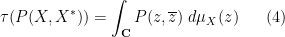
It is tempting to apply the Riesz representation theorem to (3) to define the desired measure
- In order for the polynomials to be dense in the continuous functions in the uniform topology on the support of
of
- In order for the Riesz representation theorem to apply, the functional
(or
) needs to be continuous in the uniform topology, thus one must be able to obtain a bound of the form
for some (preferably compact) set
.)
- In order to get a probability measure rather than a signed measure, one also needs some non-negativity:
needs to be non-negative whenever
for
in the intended support
To resolve the non-negativity issue, we impose an additional axiom on the non-commutative probability space
- (Non-negativity) For any
, we have
. (Note that
is self-adjoint and so its trace
is necessarily a real number.)
In the language of von Neumann algebras, this axiom (together with the normalisation
With this axiom, we can now define an positive semi-definite inner product 
This obeys the usual axioms of an inner product, except that it is only positive semi-definite rather than positive definite. One can impose positive definiteness by adding an axiom that the trace 

Without faithfulness,

In particular, we have the Cauchy-Schwarz inequality

This leads to an important monotonicity:
Exercise 2 (Monotonicity) Let
. Show that we have the monotonicity relationships
for any
.

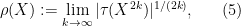
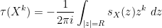
As a consequence, we can define the spectral radius 
in which case we obtain the inequality
for any
Example 3 In the case of random variables, the spectral radius is the essential supremum
, while for deterministic matrices, the spectral radius is the operator norm
. For random matrices, the spectral radius is the essential supremum
of the operator norm.
Guided by the model examples, we expect that a bounded self-adjoint element ![{[-\rho(X),\rho(X)]}](https://s0.wp.com/latex.php?latex=%7B%5B-%5Crho%28X%29%2C%5Crho%28X%29%5D%7D&bg=ffffff&fg=000000&s=0&c=20201002)

for complex numbers 

which leads to the formal Laurent series expansion
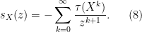
If 

We now push the domain of definition of 
Exercise 4 Let
. (Hint: use (5), (6)).
 .
.Now let 

and take Neumann series again to arrive at the formal expansion
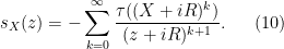
From the previous two exercises we see that

and so the above Laurent series converges for 
Exercise 6 Give a rigorous proof that the two series (8), (10) agree for
We have thus extended 


On the other hand, it is not possible to analytically extend 

for any 

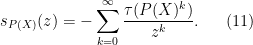
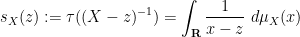
Now that we have the Stieltjes transform everywhere outside of
Proposition 7 (Boundedness) Let
![\displaystyle |\tau(P(X))| \leq \sup_{x \in [-\rho(X),\rho(X)]} |P(x)|.](https://s0.wp.com/latex.php?latex=%5Cdisplaystyle+%7C%5Ctau%28P%28X%29%29%7C+%5Cleq+%5Csup_%7Bx+%5Cin+%5B-%5Crho%28X%29%2C%5Crho%28X%29%5D%7D+%7CP%28x%29%7C.&bg=ffffff&fg=000000&s=0&c=20201002)
Proof: (Sketch) We can of course assume that 


As ![{[-\rho(P(X)),\rho(P(X))]}](https://s0.wp.com/latex.php?latex=%7B%5B-%5Crho%28P%28X%29%29%2C%5Crho%28P%28X%29%29%5D%7D&bg=ffffff&fg=000000&s=0&c=20201002)
By the previous discussion, to establish the proposition it will suffice to show that the Stieltjes transform can be continued to the domain
![\displaystyle \Omega := \{ z \in {\bf C}: z > \sup_{x \in [-\rho(X),\rho(X)]} |P(x)| \}.](https://s0.wp.com/latex.php?latex=%5Cdisplaystyle+%5COmega+%3A%3D+%5C%7B+z+%5Cin+%7B%5Cbf+C%7D%3A+z+%3E+%5Csup_%7Bx+%5Cin+%5B-%5Crho%28X%29%2C%5Crho%28X%29%5D%7D+%7CP%28x%29%7C+%5C%7D.&bg=ffffff&fg=000000&s=0&c=20201002)
For this, we observe the partial fractions decomposition

of 


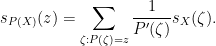
One can verify this identity is consistent with (11) for
If 


Exercise 8 Fill in the steps marked (Exercise!) in the above proof.
From Proposition 7 and the Weierstrass approximation theorem, we see that the linear functional ![{C([-\rho(X),\rho(X)])}](https://s0.wp.com/latex.php?latex=%7BC%28%5B-%5Crho%28X%29%2C%5Crho%28X%29%5D%29%7D&bg=ffffff&fg=000000&s=0&c=20201002)

Theorem 9 (Spectral theorem for bounded self-adjoint elements) Let
Remark 10 If one assumes some completeness properties of the non-commutative probability space, such as that
for other functions
than polynomials; specifically, one can do this for continuous functions
if
functions
, or square roots
, etc.. Such an assignment
is known as a functional calculus; it can be used for instance to go back and make rigorous sense of the formula (7). A functional calculus is a very convenient tool to have in operator algebra theory, and for that reason one often completes a non-commutative probability space into a
Exercise 11 Let
for all
. Conclude that the support of the spectral measure
.
![\displaystyle s_X(z) = \int_{[-\rho(X),\rho(X)]} \frac{1}{x-z}\ d\mu_X(x)](https://s0.wp.com/latex.php?latex=%5Cdisplaystyle+s_X%28z%29+%3D+%5Cint_%7B%5B-%5Crho%28X%29%2C%5Crho%28X%29%5D%7D+%5Cfrac%7B1%7D%7Bx-z%7D%5C+d%5Cmu_X%28x%29&bg=ffffff&fg=000000&s=0&c=20201002)
Exercise 12 Let
if and only if
Remark 13 It is possible to also obtain a spectral theorem for bounded normal elements along the lines of the above theorem (with
The spectral theorem more or less completely describes the behaviour of a single (bounded self-adjoint) element
- (Trace) For any two elements
.
Note that this axiom is obeyed by all three of our model examples. From this axiom, we can cyclically permute products in a trace, e.g. 


Definition 14 (Non-commutative probability space, final definition) A non-commutative probability space
From this new axiom and the Cauchy-Schwarz inequality we can now get control on products of several non-commuting elements:
Exercise 15 Let
be bounded self-adjoint elements of a tracial non-commutative probability space
for any non-negative integers
. (Hint: Induct on

Exercise 16 Let
be those elements
,
are bounded and self-adjoint; we refer to such elements simply as bounded elements. Show that this is a sub-*-algebra of
This allows one to perform the following Gelfand-Naimark-Segal (GNS) construction. Recall that 


Lemma 17 Let
with

Proof: Squaring and cyclically permuting, it will suffice to show that

Let 


By non-negativity, 

As a consequence, we see that the self-adjoint elements 

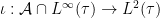
Exercise 18 (Gelfand-Naimark theorem) Show that the map
is a
, and that one has the representation
for any
is the unit vector
.
Remark 19 The Gelfand-Naimark theorem required the tracial hypothesis only to deal with the error
The Gelfand-Naimark theorem identifies 
— 2. Limits of non-commutative random variables —
One benefit of working in an abstract setting is that it becomes easier to take certain types of limits. For instance, it is intuitively obvious that the cyclic groups 


We can similarly define convergence of random variables in non-commutative probability spaces as follows.
Definition 20 (Convergence) Let
be a sequence of non-commutative probability spaces, and let
be an additional non-commutative space. For each
be a sequence of random variables in
, and let
be a sequence of random variables in
. We say that
as
. We say that
converges in the sense of moments to
.
If
, we say that

Example 21 If
converge in the sense of moments to
then we have for instance that
as
Note however that no uniformity in
), there is now no guarantee that one still has convergence.


Remark 22 When the underlying objects
. Then the constant sequence
has all the same moments as the zero random variable
, and thus converges in the sense of moments to zero, but does not converge in the
It is also clear that if we require that
For a sequence 
Exercise 23 Let
be a sequence of self-adjoint elements in non-commutative probability spaces
uniformly bounded, and let
be another bounded self-adjoint element in a non-commutative probability space
if and only if the spectral measure
converges in the vague topology to
.
Thus, for instance, one can rephrase the Wigner semi-circular law (in the convergence in expectation formulation) as the assertion that a sequence 


- A classical real random variable
.
- The identity function
in the Lebesgue space
, endowed with the trace
.
- The function
in the Lebesgue space
.
Here is a more interesting example of a semi-circular element:
Exercise 24 Let
on the natural numbers with trace
, where
is the standard basis of
. Let
be the right shift on
is a semicircular operator. (Hint: one way to proceed here is to use Fourier analysis to identify
on
, with
being the operator that maps
to
; show that
.) One can also interpret
Because we are working in such an abstract setting with so few axioms, limits exist in abundance:
Exercise 25 For each
are uniformly bounded in
and bounded self-adjoint elements
converge in moments to
. (Hint: use the Bolzano-Weierstrass theorem and the Arzelá-Ascoli diagonalisation trick to obtain a subsequence in which each of the joint moments of
converge as
— 3. Free independence —
We now come to the fundamental concept in free probability theory, namely that of free independence.
Definition 26 (Free independence) A collection
whenever
are polynomials and
equal.
A sequence
is asymptotically freely independent (or asymptotically free for short) if one has
as


Remark 27 The above example describes freeness of collections of random variables
Thus, for instance, if 


To contrast free independence with classical independence, suppose that 

For a trivial example of free independence,
Exercise 28 Suppose that
.)
A less trivial example of free independence comes from the free group, which provides a clue as to the original motivation of this concept:
Exercise 29 Let
. Let
be the non-commutative probability space of bounded linear operators on the Hilbert space
, with trace
, where
is the Kronecker delta function at the identity. Let
be the shift operators
for
and
. Show that
are freely independent.

For classically independent commuting random variables 


Expanding this using linear nature of trace, one soon sees that

So far, this is just as with the classically independent case. Next, we consider a slightly more complicated moment, 


In the classically independent case, we can conclude the latter term would vanish. We cannot immediately say that in the freely independent case, because only one of the factors has mean zero. But from (12) we know that 

and now free independence does ensure that this term vanishes, and so

So again we have not yet deviated from the classically independent case. But now let us look at 


From (13) we have 

Now we split 


which simplifies to

which differs from the classical independence prediction of 
This process can be continued:
Exercise 30 Let
of the
. (Hint: induct on the complexity of the moment.)
The product measure construction allows us to generate classically independent random variables at will (after extending the underlying sample space): see Exercise 18 of Notes 0. There is an analogous construction, called the amalgamated free product, that allows one to generate families of freely independent random variables, each of which has a specified distribution. Let us give an illustrative special case of this construction:
Lemma 31 (Free products) For each
, let
be a non-commutative probability space. Then there exists a non-commutative probability space
for
, then
Proof: (Sketch) Recall that each 


We now form the Fock space 
where 


when 


when 


Exercise 32 Complete the proof of Lemma 31. (Hint: you may find it helpful to first do Exercise 29, as the construction here is in an abstraction of the one in that exercise.)
Finally, we illustrate the fundamental connection between free probability and random matrices observed by Voiculescu, namely that (classically) independent families of random matrices are asymptotically free. The intuition here is that while a large random matrix 


We give a typical instance of this phenomenon here:
Proposition 33 (Asymptotic freeness of Wigner matrices) Let
be a collection of independent
moments for each
. Then the random variables
are asymptotically free.
Proof: (Sketch) Let us abbreviate 


for each fixed choice of natural numbers 

Recall from Notes 3 that 


One can perform a similar computation to compute 


Exercise 34 Expand the above sketch into a full proof of the above theorem.
Remark 35 This is by no means the only way in which random matrices can become asymptotically free. For instance, if instead one considers random matrices of the form
, where
are deterministic Hermitian matrices with uniformly bounded eigenvalues, and the
are iid unitary matrices drawn using Haar measure on the unitary group
, one can also show that the
are asymptotically free; again, see the paper of Voiculescu for details.
— 4. Free convolution —
When one is summing two classically independent (real-valued) random variables 


by means of the simple formula

As we saw in Notes 2, this can be used in particular to establish a short proof of the central limit theorem.
There is an analogous theory when summing two freely independent (self-adjoint) non-commutative random variables 
which has already been discussed earlier.
Here’s how to use this transform to compute free convolutions. If one wishes, one can that
The trick (which we already saw in Notes 4) is not to view 


With this inversion, we thus have


for some 

Similarly we have

and so
![\displaystyle X + Y = z_X(s) + z_Y(s) + s^{-1} [ (1-E_X)^{-1} + (1-E_Y)^{-1} ].](https://s0.wp.com/latex.php?latex=%5Cdisplaystyle+X+%2B+Y+%3D+z_X%28s%29+%2B+z_Y%28s%29+%2B+s%5E%7B-1%7D+%5B+%281-E_X%29%5E%7B-1%7D+%2B+%281-E_Y%29%5E%7B-1%7D+%5D.&bg=ffffff&fg=000000&s=0&c=20201002)
We can combine the second two terms via the identity

Meanwhile

and so
![\displaystyle X + Y = z_X(s) + z_Y(s) + s^{-1} + s^{-1} [(1-E_X)^{-1} (1 - E_X E_Y) (1-E_Y)^{-1}].](https://s0.wp.com/latex.php?latex=%5Cdisplaystyle+X+%2B+Y+%3D+z_X%28s%29+%2B+z_Y%28s%29+%2B+s%5E%7B-1%7D+%2B+s%5E%7B-1%7D+%5B%281-E_X%29%5E%7B-1%7D+%281+-+E_X+E_Y%29+%281-E_Y%29%5E%7B-1%7D%5D.&bg=ffffff&fg=000000&s=0&c=20201002)
We can rearrange this a little bit as
![\displaystyle (X+Y - z_X(s)-z_Y(s)-s^{-1})^{-1} = s [(1-E_Y) (1 - E_X E_Y)^{-1} (1-E_X) ].](https://s0.wp.com/latex.php?latex=%5Cdisplaystyle+%28X%2BY+-+z_X%28s%29-z_Y%28s%29-s%5E%7B-1%7D%29%5E%7B-1%7D+%3D+s+%5B%281-E_Y%29+%281+-+E_X+E_Y%29%5E%7B-1%7D+%281-E_X%29+%5D.&bg=ffffff&fg=000000&s=0&c=20201002)
We expand out as (formal) Neumann series:

This expands out to equal 

Now we use the hypothesis that

and so

Comparing this against (15) for

Thus, if we define the 
then we have the addition formula
Since one can recover the Stieltjes transform 
For comparison, we have the (formal) addition formula

for classically independent real random variables
Exercise 36 Let
where the cumulants
can be reconstructed from the moments
for
. (Hint: start with the identity
.) Thus for instance
is the expectation,
is the variance, and the third and fourth cumulants are given by the formula
Establish the additional formula
where
ranges over all partitions of
into non-empty cells
.


Exercise 37 Let
where the free cumulants
can be reconstructed from the moments
for
.) Thus for instance
is the expectation,
is the variance, and the third and fourth free cumulants are given by the formulae
Establish the additional formula
where
lie in
lie in one cell
lie in a distinct cell
.


Remark 38 These computations illustrate a more general principle in free probability, in that the combinatorics of free probability tend to be the “non-crossing” analogue of the combinatorics of classical probability; compare with Remark 7 of Notes 3.
Remark 39 The
-transform, for computing the spectral behaviour (or more precisely, the joint moments) of products
of free random variables; see for instance these notes of Speicher.
The
Exercise 40 Let
for any
. In particular, the free convolution of
and
is
.
Exercise 41 From the above exercise, we see that the effect of adding a free copy of
. Explain how this is compatible with the Dyson Brownian motion computations in Notes 4.
It also gives a free analogue of the central limit theorem:
Exercise 42 (Free central limit theorem) Let
and
), and let
be free copies of
. Show that the coefficients of the formal power series
converge to that of the identity function
converges in the sense of moments to a semi-circular element
The free central limit theorem implies the Wigner semi-circular law, at least for the GUE ensemble and in the sense of expectation. Indeed, if 

On the other hand, if 


54 comments
Comments feed for this article
11 February, 2010 at 5:08 am
Johan
In example 1 I believe there are a few places where has become
  because of typos.
Specifically, I believe the range of the multiplication operation should be , that this should also be both the domain and the range of the involution operation and that the expectation operator is a linear operator on
[Corrected, thanks – T.]
12 February, 2010 at 6:18 pm
George Lowther
I don’t know if I’m misunderstanding something here, but in Exercise 1 I don’t see any reason why the sequence should be non-decreasing. If X was a centered Gaussian, or any other symmetric RV, then it will be zero for odd k and positive and non-decreasing for even k.
12 February, 2010 at 7:08 pm
Terence Tao
Ah, right, the monotonicity is only partial for the odd moments (the odd moments are bounded by the next even moment, but not vice versa). I’ve changed the text accordingly.
13 February, 2010 at 6:53 am
George Lowther
Also, I think you should have exponent of k+1 rather than k in the denominator in expressions (8),(10),(11) for s_X.
[Corrected, thanks – T.]
13 February, 2010 at 12:18 am
Greg Kuperberg
In the non-commutative setting, the correct notion is now of two (bounded, self-adjoint) non-commutative random variables {X, Y} being freely independent (or free for short)
I would say a correct, not the correct. If you accept von Neumann algebras and C*-algebras, but instead retain ordinary commutative independence, then the theory is standard quantum probability. In the context of empirical science, standard quantum probability is more often correct than classical probability (which it generalizes), and it is far more often correct than free probability (whose relevance to physics is credible but speculative).
However, we will proceed here instead by working with a (possibly incomplete) non-commutative probability space, and working primarily with formal expressions (e.g. formal power series in z) without trying to evaluate such expressions in some completed space.
This amounts to reducing all probability to a theory of moments. This has led to all sorts of confusion in parts of the literature in quantum probability. Everyone understands that a classical distribution has more information in it than just its moments; thus axioms based only on moments aren’t very good axioms. The same thing happens in non-commutative probability of course. The only reason that this simplification is somewhat accountable in free probability is that typical limit laws (like the Wigner semicircle) are bounded. Of course this is not true in standard quantum probability, which again is non-commutative but with a commutative independence law. (It’s also not a full excuse to just look at moments, although you seem to acknowledge that completions could be important later.)
So I would put a stronger disclaimer here.
13 February, 2010 at 8:46 am
Terence Tao
Fair enough; I’ve amended the text accordingly.
Quantum observables, while not exactly commutative in general, are still often approximately commutative, thanks to the correspondence principle, which is why classical independence is still a useful concept; in contrast, a pair of random matrices tends to be “maximally non-commutative”, making free probability the more relevant concept. So in some sense they represent the two opposite extremes of non-commutative probability.
It’s also true that the moment-centric viewpoint of free probability, which makes computations purely algebraic in nature rather than analytic, breaks down for unbounded variables, which of course occur all the time in quantum mechanics. I mention this restriction to bounded variables in the introduction.
13 February, 2010 at 11:09 am
Greg Kuperberg
Quantum observables, while not exactly commutative in general, are still often approximately commutative, thanks to the correspondence principle, which is why classical independence is still a useful concept
I have really learned something from this remark: Although I always knew that commutative independence (as opposed to free independence) is still important in quantum probability, I didn’t consider that you would want a dynamical reason to justify it. That said, I only half agree with you. One reason that commutative independence is still relevant in physics is indeed that we live in a semiclassical regime of the laws of physics. (So when you say “often”, it is in the same sense that if we were fish, we would think that 3-dimensional regions are “often” filled with water.)
But two other reasons that commutative independence are relevant in quantum probability are (1) finite communication speed, and (2) weak coupling. These two reasons, and not the semiclassical limit, are why quantum computation is premised on standard quantum probability rather than (say) free probability. One of the things that I did not realize, and which is definitely useful to say, is that in the human realm (again, if we were fish…), is that neither finite communication speed nor weak coupling are directly the point. If the price of groceries in Atlanta is statistically independent from the distribution of potholes in Seattle, it isn’t because of a bound on the speed of light or sound, nor a bound the strength of the electromagnetic field. Instead, there is an emergent statistical weak coupling, which is related to the emergent classical/semiclassical regime that we live in.
Actually, I guess there are also examples of emergent weak coupling in quantum physics. They are associated with classical limits, but that is not strictly necessary.
As you imply, free probability could be a relevant model when quantum random variables are as interdependent as possible. The nuclear physics motivation of random matrix theory reflects this. Voiculescu also told me that free probability models large N gauge theory, presumably for similar reasons.
13 February, 2010 at 7:01 am
Anonymous
Dear Prof. Tao,
How do we define infinite products?
is the limit of partial products?
Thanks
16 February, 2010 at 6:00 am
Anonymous
Yes
29 June, 2014 at 12:17 am
Labair Abdelkader
See here http://en.wikipedia.org/wiki/Infinite_product
16 February, 2010 at 2:35 pm
Jérôme Chauvet
Dear Pr. Tao,
In section: 3. Free Independence (in the text right after Remark5), I see you wrote “vanish” twice instead of once.
Regards,
[Corrected, thanks – T.]
17 February, 2010 at 5:25 am
Jérôme Chauvet
Dear Pr. Tao,
There is an important loss, in section 3 again (at least with Explorer). In the definition box #7 of free independence, the right hand side term in the limit, i.e., the limit condition on tau for a sequence of variables to be asymptotically free, is out of the box, so one cannot read it at all.
Best,
[Corrected, thanks – T.]
26 February, 2010 at 9:59 pm
mmailliw/william
In the proof of Theorem 2, you decompose 1/(P(w) – z) as the sum of
(P'(zeta))^(-1)/(w – zeta), summing over the values of zeta for which P(zeta) = z.
After integrating, you then conclude that ‘formally’,
s_(P(X))(z) = Sigma[1/(P'(zeta)) s_X(z)], summing over zeta with P(zeta) = z.
However, I’m wondering whether the s_X(z) should actually be an s_X(zeta). After all, we know that zeta lies outside the interval [-rho(X), rho(X)], so s_X is defined on zeta, but we don’t seem to have this same guarantee for z!
(In other words, should the formal formula really be
s_(P(X))(z) = Sigma[1/(P'(zeta)) s_X(zeta)]?)
[Corrected, thanks – T.]
8 March, 2010 at 7:19 am
Brian Davies
The heavy emphasis on the use of the trace in these notes reminds me of the theory of Hilbert algebras in Jacques Dixmier’s very old Operator Algebra book Chapter 1 section 5 and in his C*-algebra book Chapter 13. Algebras with traces are very special and have a correspondingly nice mathematical theory.
In quantum statistical mechanics it has been found that the non-commutative algebras involved do not have natural traces (except in the case of infinite temperature) and the corresponding theory involves Type 3 von Neumann algebras. The trace condition is replaced by a KMS condition, but it seems hard to define this in your purely algebraic context.
8 March, 2010 at 2:28 pm
Sungjin Kim
In exercise 2, it seems that (5) and (6) give only = ?
8 March, 2010 at 2:33 pm
Sungjin Kim
In exercise 2, it seems (5) and (6) give only $\leq$, and it is enough for the rest of argument. How is it possible to obtain $\geq$ ?
p.s. $\leq$ and $\geq$ has been disappeared in previous comment because of HTML..
10 March, 2010 at 5:37 pm
Terence Tao
From (5), we have whenever k is even and sufficiently large depending on
  . This is enough to obtain the lower bound (though, as you say, it is not strictly necessary to have this bound for the application at hand).
14 March, 2010 at 11:33 am
254A, Notes 8: The circular law « What’s new
[…] failure of the moment method also shows that methods of free probability (Notes 5) do not work directly. For instance, observe that for fixed , and (in the noncommutative […]
31 March, 2010 at 3:32 pm
wang
Maybe the title “245A, Notes 5: Free probability” should be “254A …”. When I search your
245A notes in google (terrytao 245a), I get here :-)
[Corrected, thanks – T.]
2 June, 2010 at 5:33 pm
Aaron F.
Maybe it’s just my browser (Firefox 3.0.19), but some of the displayed equations seem to be missing! I’ve noticed gaps in the following places:
“The measure {\mu_X} is related to the moments {\tau(X^k) = \mathop{\mathbb E} X^k} by the formula…”
“it is natural to try to define this measure through the formula (1), or equivalently (by linearity) through the formula…”
“In fact, one has the more general formula…”
“In the normal case, one may hope to work with the more general formula…”
“we can define the spectral radius {\rho(X)} of a self-adjoint element {X} by the formula…”
“in which case we obtain the inequality…”
[Fixed, thanks – T.]
p.s. Even with missing equations, these notes are wonderful. :)
30 July, 2010 at 10:37 pm
Anonymous
It could be my browser, but I think there is a missing “1/2” in
is a semi-definite inner product space with semi-norm
[]:=(_{L^2(\tau)})^{1/2}=[]
[Corrected, thanks – T.]
2 August, 2010 at 7:14 pm
Anonymous
It seems like the last modification change some latex code, because the numered equation are missing and the equations are not centered.
[Fixed, thanks – T.]
4 August, 2010 at 10:04 pm
Anonymous
I have notice some typos (if I’m not misunderstanding something).
In the definition of spectral radius the exponent is 1/(2K) [instead 1/2k].
In Exercise 6 the formula must say \mu_X(x) [instead \mu_X(z)].
I think that the right side of the equation that follows “cyclic property of trace and induction.) We conclude that” must be 1. The next equation shouldn’t be \tau(…)=s?
In the last formula of exercise 20, you use \kappa instead C (but using C we have two letters C, for free cumulants and for cells).
In remark 8, I think there is a missing link in “these notes of Speicher”.
[Corrected, thanks – T.]
Nice notes, I learned a lot. Thanks!
10 August, 2010 at 6:13 pm
Anonymous
In the last formula of exercise 20, kappa is used for free cumulants, while the right letter is C.
Thanks a lot.
[Corrected, thanks – T.]
30 November, 2010 at 8:29 pm
Free Probability | Honglang Wang's Blog
[…] link about the survey of free probability. I hope it will be useful for you. Terry Tao also have a post about […]
3 March, 2011 at 10:11 am
FP Recent Follows « YW's E-Profile
[…] https://terrytao.wordpress.com/2010/02/10/245a-notes-5-free-probability/ […]
19 June, 2011 at 1:11 pm
Jérôme Chauvet
Dear Pr. Tao,
What if one is considering a setting {A,B}, with A and B being 2 (real-valued) sqaure matrices that do not commute with each other + a composition law on this set + a recursion that chooses at random for each step the multiplication order according to a Bernouilli law as follows:
u(n+1) = ABu(0) or u(n+1) = BAu(0)
I guess one instance of the recursion up to p (amongst 2^p of them) would look like:
u(n+p) = ABBABAAB….BAu(0)
And it would be akin to some sort of chaotic matrix K such that:
u(n+p) = K u(0) where X=ABBABAAB….BA
Though being not properly a random matrix (I mean matrices for which coefficients are gaussian variables…)
The question is: Would the probability measure of this system attainable by the theory you are presenting here?
Thanks a lot :)
20 June, 2011 at 10:38 am
Terence Tao
Random products of fixed matrices are well studied, being related to random walks on groups and expander graphs, but the regime studied (long products of small matrices) is different from the one where free probability is useful (short products of large matrices) and other tools are used instead (entropy, representation theory, spectral gaps, etc.).
27 March, 2012 at 7:00 am
Anonymous
Prof Tao,
Scalar (commutative) random variables should be a special case of non-commutative random variables, so I think that in this special case the two kinds of convolutions should be the same? But then we would have two central limit theorem with two different limit distribution?
27 March, 2012 at 7:15 am
Anonymous
Also, if A is a symmetric matrix, with entries i.i.d. Gaussian, the distribution of it is NOT the semicircle law. Then we take sum of n copies of it and divided by square root of n, and we get the same matrix, but on the other hand it converges to semicircle law?
I guess there is something fundamental that I misunderstood.
27 March, 2012 at 8:17 am
Anonymous
Sorry I read your notes again, and found that freeness is not the same with independence even in the commuting case! Please ignore my question!
18 August, 2012 at 9:06 pm
Noncommutative probability « Annoying Precision
[…] noncommutative probability provides such an approach. Terence Tao’s notes on free probability develop a version of noncommutative probability approach geared towards applications to random […]
25 October, 2012 at 10:11 am
Walsh’s ergodic theorem, metastability, and external Cauchy convergence « What’s new
[…] any , which we will use in the sequel without further comment; see e.g. these previous blog notes for proofs. (Actually, for the purposes of proving Theorem 3, one can specialise to the case (and […]
14 February, 2014 at 6:01 am
shubhashedthikere
Prof Tao,
I needed clarification regarding Example 3: Random matrix variables. Here is the space of random matrices a tensor product of the vector space L^{\infty-}( which is infinite dimensional) and (finite dimensional) vector space M_n({\bf C})? If yes, could you please tell me how would a tensor product for an infinite dimensional vector space is defined?
If {X \in L^{\infty-} \otimes M_n({\bf C})}, is not tensor product, then, could you please explain what exactly is this space of random matrices?
14 February, 2014 at 9:27 am
Terence Tao
If is an infinite-dimensional vector space and
  is a finite-dimensional vector space, one can define the tensor product by selecting a basis
  for
for  and defining
  to be the set of all formal vectors of the form
  with
with  , with the vector space operations defined in the obvious manner. This defines a vector space
  with a bilinear tensor product
  which obeys the usual tensor product axioms, and up to isomorphism this space does not depend on the choice of basis
  .
.
In the specific case , this construction gives the space of
  matrices whose entries are all in
  , i.e. random matrices with all moments finite.
28 June, 2014 at 10:22 pm
Algebraic probability spaces | What's new
[…] probability space, and is very similar to the non-commutative probability spaces studied in this previous post, except that these spaces are now commutative (and […]
28 June, 2014 at 11:51 pm
Mustafa Said
Is there a version of the Erdos probabilistic method in the non-commutative setting?
16 April, 2015 at 11:09 pm
Anonymous
Could I ask for some hint to prove the first inequality in Exercise 3? My idea was to write the normal operator in terms of the bounded self-adjoint and commuting real and imaginary components. For the first two values of the exponent (1 and 2) it follows from the obvious identities (including Schwarz inequality). The case when the exponent is 3 or 4 has already some issues: some generalized (or perhaps smarter) versions of Schwarz inequality seem to be needed. I can handle the case 3 but the case 4 is even harder. Any suggestion?
17 April, 2015 at 8:02 am
Terence Tao
If is normal, then
  .
.
28 March, 2017 at 3:12 pm
tornado92
A few typos: In Exercises 19 and 20, the final “additional formulas” seem to be swapped. Also, I think the formula for the third cumulant should actually be equal to the formula given for the third free cumulant. I guess they start differing at …
…
[Corrected, thanks – T.]
25 May, 2017 at 2:19 pm
Ranjan
The Expected value of f(X) not necessarily 0 for being independent with Y, please change the above notation.
31 August, 2017 at 1:03 pm
numberoftargets
It is never mentioned that expected of f(X) needs to be 0 for being independent with Y.
31 August, 2017 at 6:03 am
burakcakmakblog
Professor, In section 4 (i.e. Free convolution), how do you guarantee that we can expand into a (formal) Neumann series? Because it requires that
  has the bounded eigenvalues below one.
31 August, 2017 at 8:27 am
Terence Tao
A formal series does not require the partial sums to converge; in particular, a formal Neumann series such as is well-defined even if
  has spectral radius larger than 1.
16 September, 2017 at 2:08 pm
Inverting the Schur complement, and large-dimensional Gelfand-Tsetlin patterns | What's new
[…] these previous notes for a discussion of free probability topics such as the […]
27 April, 2018 at 2:34 pm
tornado92
Possible typo: Example 3 states that for deterministic matrices, the spectral radius is the operator norm. This seems false–for example, what if the matrix is nilpotent? Then the spectral radius is zero, but the operator norm could easily be nonzero. I guess you need the matrix to be normal for this to work.
Another question: For bounded operators on a Hilbert space, there is already an existing notion of spectral radius, which is simply the radius of the smallest disc containing the spectrum. It turns out this is the limit of the kth root of the operator norm of the kth power, as k goes to infinity. However, in these notes, the spectral radius is defined in terms of the state. So my question is, is the spectral radius independent of the state you choose? If not, is there a state for which you recover the existing notion of spectral radius?
29 April, 2018 at 1:22 pm
Terence Tao
In these notes the spectral radius is only defined for self-adjoint elements. In the case where the noncommutative probability space is a space of bounded operators on a Hilbert space with trace given by a state, the spectral radius on this noncommutative space will always be bounded by the operator norm, and one will have equality as long as the state has a nontrivial component at the edge of the spectrum of the Hilbert space operator.
1 November, 2018 at 8:22 am
tpfly
Dear Mr. Tao,
I think I’ve found a counterexample of Exercise 28 (if I didn’t misunderstand the concept of free independence). Take iid random variables uniformly distributed on the unit circle, with
  . then for any polynomial P,
  iff
iff  .
.
Now suppose ,
,  are polynomials without constant term, then we have
 . As defined,
  are freely independent. But they are not scalars.
Maybe in the definition of free independence we should be able to take in the polynomials?
[Oops, I meant to insert the hypothesis that are self-adjoint -T.]
4 September, 2019 at 11:30 am
Bharath Krishnan
Dear Professor Tao,
This does not directly address your post but is related to probability/measure theory. Measure theory, for continuous functions, has always been based on intuition. Currently, the most intuitive and well-known measure of functions defined in![[a,b]\cap\mathbb{R}](https://s0.wp.com/latex.php?latex=%5Ba%2Cb%5D%5Ccap%5Cmathbb%7BR%7D&bg=ffffff&fg=545454&s=0&c=20201002) , is the Lebesgue measure. However, when the Lebesgue measure of a function’s domain, defined on a subset of
, is the Lebesgue measure. However, when the Lebesgue measure of a function’s domain, defined on a subset of ![[a,b]](https://s0.wp.com/latex.php?latex=%5Ba%2Cb%5D&bg=ffffff&fg=545454&s=0&c=20201002) is zero, the average could be outside the infimum and supremum of the function’s range. Since the average is strongly related to the measure and integration, we can say the Lebesgue measure is not intuitive enough.
is zero, the average could be outside the infimum and supremum of the function’s range. Since the average is strongly related to the measure and integration, we can say the Lebesgue measure is not intuitive enough.
If the Lebesgue measure is not intuitive enough what is an intuitive, unique average of a function on any domain.
There is a website below-showing intuitions and measures that I and other people think are alternatives to Lebesgue measure when the measure of the domain is zero.
https://math.stackexchange.com/questions/3329506/most-intuitive-average-of-p-for-all-x-in-a-cap-a-b-where-a-subseteq-m
8 December, 2019 at 3:47 pm
States on *-Algebras | Almost Sure
[…] the semi-norm defined above. Interestingly, Terry Tao uses exactly this definition of the norm in his posts on NC probability, although he does concentrate on tracial […]
26 December, 2021 at 3:48 pm
co.combinatorics - Combinatorial/diagrammatic fashions totally free significance partition polynomials Answer - Lord Web
[…] relationships“by Ebrahimi-Fard, Foissy, Kock and Patras; Ex. 37 by Terry Tao’s Notes on free chance; and P. 22 of “Enumeration geometry, tau capabilities and Heisenberg-Virasoro […]
31 December, 2021 at 5:57 pm
co.combinatorics - Combinatorics for the motion of Virasoro / Kac-Schwarz operators: partition polynomials of free chance principle Answer - Lord Web
[…] relationships“by Ebrahimi-Fard, Foissy, Kock and Patras; Ex. 37 by Terry Tao’s Notes on free chance; and P. 22 of “Enumeration geometry, tau features and Heisenberg-Virasoro algebra“by […]
8 January, 2022 at 12:19 pm
Tom Copeland
The previous two spam pingbacks from Lord Web contain corrupted copies of my MO-Q that completely algebraically characterizes the transformations between the free cumulants and moments for the single variable case, an alternative to Ex. 37 above, related to Kac-Schwarz operators. Correct version: Combinatorics for the action of Virasoro / Kac–Schwarz operators: partition polynomials of free probability theory
6 August, 2022 at 12:55 pm
What is the trace? – Alexander Van Werde
[…] probability theory is a beautiful subject but it would lead us too far to go into detail here. See this blog post by Terrence Tao or the list of literature on Roland Speicher’s blog if you wish to […]