
This is going to be a somewhat experimental post. In class, I mentioned that when solving the type of homework problems encountered in a graduate real analysis course, there are really only about a dozen or so basic tricks and techniques that are used over and over again. But I had not thought to actually try to make these tricks explicit, so I am going to try to compile here a list of some of these techniques here. But this list is going to be far from exhaustive; perhaps if other recent students of real analysis would like to share their own methods, then I encourage you to do so in the comments (even – or especially – if the techniques are somewhat vague and general in nature).
(See also the Tricki for some general mathematical problem solving tips. Once this page matures somewhat, I might migrate it to the Tricki.)
Note: the tricks occur here in no particular order, reflecting the stream-of-consciousness way in which they were arrived at. Indeed, this list will be extended on occasion whenever I find another trick that can be added to this list.
1. Split up equalities into inequalities.
If one has to show that two numerical quantities X and Y are equal, try proving that 

In a similar spirit, to show that two sets E and F are equal, try proving that 

2. Give yourself an epsilon of room.
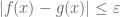
If one has to show that 

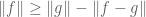
In a similar spirit, if one needs to show that a quantity 

Or: if one wishes to show that two functions 

Or: if one wants to show that a sequence 

Don’t be too focused on getting all your error terms adding up to exactly 


One caveat: for finite 


See also the Tricki article on this topic.
3. Decompose or approximate a rough or general object by a smoother or simpler one.
If one has to prove something about an unbounded (or infinite measure) set, consider proving it for bounded (or finite measure) sets first if this looks easier.
Similarly:
- if one has to prove something about a measurable set, try proving it for open, closed, compact, bounded, or elementary sets first.
- if one has to prove something about a measurable function, try proving it for functions that are continuous, bounded, compactly supported, simple, absolutely integrable, etc.
- if one has to prove something about an infinite sum or sequence, try proving it first for finite truncations of that sum or sequence (but try to get all the bounds independent of the number of terms in that truncation, so that you can still pass to the limit!).
- if one has to prove something about a complex-valued function, try it for real-valued functions first.
- If one has to prove something about a real-valued function, try it for unsigned functions first.
- If one has to prove something about a simple function, try it for indicator functions first.
In order to pass back to the general case from these special cases, one will have to somehow decompose the general object into a combination of special ones, or approximate general objects by special ones (or as a limit of a sequence of special objects). In the latter case, one may need an epsilon of room (trick 2), and some sort of limiting analysis may be needed to deal with the errors in the approximation (it is not always enough to just “pass to the limit”, as one has to justify that the desirable properties of the approximating object are preserved in the limit).
Note: one should not do this blindly, as one might then be loading on a bunch of distracting but ultimately useless hypotheses that end up being a lot less help than one might hope. But they should be kept in mind as something to try if one starts having thoughts such as “Gee, it would be nice at this point if I could assume that 
In the more quantitative areas of analysis and PDE, one sees a common variant of the above technique, namely the method of a priori estimates. Here, one needs to prove an estimate or inequality for all functions in a large, rough class (e.g. all rough solutions to a PDE). One can often then first prove this inequality in a much smaller (but still “dense”) class of “nice” functions, so that there is little difficulty justifying the various manipulations (e.g. exchanging integrals, sums, or limits, or integrating by parts) that one wishes to perform. Once one obtains these a priori estimates, one can then often take some sort of limiting argument to recover the general case.
4. If one needs to flip an upper bound to a lower bound or vice versa, look for a way to take reflections or complements.
Sometimes one needs a lower bound for some quantity, but only has techniques that give upper bounds. In some cases, though, one can “reflect” an upper bound into a lower bound (or vice versa) by replacing a set 


The triangle inequality
can be used to flip an upper bound on 


can flip a upper bound on 
5. Uncountable unions can sometimes be replaced by countable or finite unions.
Uncountable unions are not well-behaved in measure theory; for instance, an uncountable union of null sets need not be a null set (or even a measurable set). (On the other hand, the uncountable union of open sets remains open; this can often be important to know.) However, in many cases one can replace an uncountable union by a countable one. For instance, if one needs to prove a statement for all 
In a similar spirit, given a real parameter 
If you are working on a compact set, then one can often replace even uncountable unions with finite ones, so long as one is working with open sets. When this option is available, it is often worth spending an epsilon of measure (or whatever other resource is available to spend) to make one’s sets open, just so that one can take advantage of compactness.
6. If it is difficult to work globally, work locally instead.
A domain such as Euclidean space 


7. Be willing to throw away an exceptional set.
The “Lebesgue philosophy” to measure theory is that null sets are often “irrelevant”, and so one should be very willing to cut out a set of measure zero on which bad things are happening (e.g. a function is undefined or infinite, a sequence of functions is not converging, etc.). One should also be only slightly less willing to throw away sets of positive but small measure, e.g. sets of measure at most
Many things in measure theory improve after throwing away a small set. The most notable examples of this are Egorov’s theorem (pointwise a.e. convergence becomes locally uniform convergence after throwing away a small set) and Lusin’s theorem (measurable functions become continuous after throwing away a small set). A related (and simpler) principle is that a measurable function 


A little later in this course, we will also start seeing a similar trick of throwing away most of a sequence and working with a subsequence instead. (This trick can also be interpreted as “throwing away a small set”, but to understand what “small” means in this context, one needs the language of ultrafilters, which will not be discussed here.) See Trick 17 below.
8. Draw pictures and try to build counterexamples.
Measure theory, particularly on Euclidean spaces, has a significant geometric aspect to it, and you should be exploiting your geometric intuition. Drawing pictures and graphs of all the objects being studied is a good way to start. These pictures need not be completely realistic; they should be just complicated enough to hint at the complexities of the problem, but not more. (For instance, usually one- or two-dimensional pictures suffice for understanding problems in
A common mistake is to try to draw a picture in which both the hypotheses and conclusion of the problem hold. This is actually not all that useful, as it often does not reveal the causal relationship between the former and the latter. One should try instead to draw a picture in which the hypotheses hold but for which the conclusion does not – in other words, a counterexample to the problem. Of course, you should be expected to fail at this task, given that the statement of the problem is presumably true. However, the way in which your picture fails to accomplish this task is often very instructive, and can reveal vital clues as to how the solution to the problem is supposed to proceed.
9. Try simpler cases first.
This advice of course extends well beyond measure theory, but if one is completely stuck on a problem, try making the problem simpler (while still capturing at least one of the difficulties of the problem that you cannot currently resolve). For instance, if faced with a problem in 

The problem should not be made so simple that it becomes trivial, as this doesn’t really gain you any new insight about the original problem; instead, one should try to keep the “essential” difficulties of the problem while throwing away those aspects that you think are less important (but are still serving to add to the overall difficulty level).
On the other hand, if the simplified problem is unexpectedly easy, but one cannot extend the methods to the general case (or somehow leverage the simplified case to the general case, as in Trick 3), this is an indication that the true difficulty lies elsewhere. For instance, if a problem involving general functions could be solved easily for monotone functions, but one cannot then extend that argument to the general case, this suggests that the true enemy is oscillation, and perhaps one should try another simple case in which the function is allowed to be highly oscillatory (but perhaps simple in other ways, e.g. bounded with compact support).
10. Abstract away any information that you believe or suspect to be irrelevant.
Sometimes one is faced with an embarrassment of riches when it comes to what choice of technique to use on a problem; there are so many different facts that one knows about the problem, and so many different pieces of theory that one could apply, that one doesn’t quite know where to begin.
When this happens, abstraction can be a vital tool to clear away some of the conceptual clutter. Here, one wants to “forget” part of the setting that the problem is phrased in, and only keep the part that seems to be most relevant to the hypotheses and conclusions of the problem (and thus, presumably, to the solution as well).
For instance, if one is working in a problem that is set in Euclidean space
[It is worth noting that sometimes this abstraction method does not always work; for instance, when viewed as a measure space, 
Another example of abstraction: suppose that a problem involves a large number of sets (e.g. 


A real-life example: a student once asked me how to justify the claim that
uniformly for 


At this point it is clear what to do: use Taylor’s theorem with remainder.
Note that this trick is in many ways the antithesis of Trick 9, because by passing to a special case, one often makes the problem more concrete, with more things that one is now able to start trying. However, the two tricks can work together. One particularly useful “advanced move” in mathematical problem solving is to first abstract the problem to a more general one, and then consider a special case of that more abstract problem which is not directly related to the original one, but is somehow simpler than the original while still capturing some of the essence of the difficulty. Attacking this alternate problem can then lead to some indirect but important ways to make progress on the original problem.
11. Exploit Zeno’s paradox: a single epsilon can be cut up into countably many sub-epsilons.
A particularly useful fact in measure theory is that one can cut up a single epsilon into countably many pieces, for instance by using the geometric series identity

this observation arguably goes all the way back to Zeno. As such, even if one only has an epsilon of room budgeted for a problem, one can still use this budget to do a countably infinite number of things. This fact underlies many of the countable additivity and subadditivity properties in measure theory, and also makes the ability to approximate rough objects by smoother ones to be useful even when countably many rough objects need to be approximated.
In general, one should be alert to this sort of trick when one has to spend an epsilon or so on an infinite number of objects. If one was forced to spend the same epsilon on each object, one would soon end up with an unacceptable loss; but if one can get away with using a different epsilon each time, then Zeno’s trick comes in very handy.
Needless to say, this trick combines well with Trick 2.
12. If you expand your way to a double sum, a double integral, a sum of an integral, or an integral of a sum, try interchanging the two operations.
Or, to put it another way: “The Fubini-Tonelli theorem is your friend”. Provided that one is either in the unsigned or absolutely convergent worlds, this theorem allows you to interchange sums and integrals with each other. In many cases, a double sum or integral that is difficult to sum in one direction can become easier to sum (or at least to upper bound, which is often all that one needs in analysis). In fact, if in the course of expanding an expression, you encounter such a double sum or integral, you should reflexively try interchanging the operations to see if the resulting expression looks any simpler.
Note that in some cases the parameters in the summation may be constrained, and one may have to take a little care to sum it properly. For instance,

interchanges (assuming that the 

(why? try plotting the set of pairs 

(extending the domain of 
The following point is obvious, but bears mentioning explicitly: while the interchanging sums/integrals trick can be very powerful, one should not apply it twice in a row to the same double sum or double operation, unless one is doing something genuinely non-trivial in between those two applications. So, after one exchanges a sum or integral, the next move should be something other than another exchange (unless one is dealing with a triple or higher sum or integral).
A related move (not so commonly used in measure theory, but occurring in other areas of analysis, particularly those involving the geometry of Euclidean spaces) is to merge two sums or integrals into a single sum or integral over the product space, in order to use some additional feature of the product space (e.g. rotation symmetry) that is not readily visible in the factor spaces. The classic example of this trick is the evaluation of the gaussian integral 
13. Pointwise control, uniform control, and integrated (average) control are all partially convertible to each other.
There are three main ways to control functions (or sequences of functions, etc.) in analysis. Firstly, there is pointwise control, in which one can control the function at every point (or almost every point), but in a non-uniform way. Then there is uniform control, where one can control the function in the same way at most points (possibly throwing out a set of zero measure, or small measure). Finally, there is integrated control (or control “on the average”), in which one controls the integral of a function, rather than the pointwise values of that function.
It is important to realise that control of one type can often be partially converted to another type. Simple examples include the deduction of pointwise convergence from uniform convergence, or integrating a pointwise bound 

14. If the conclusion and hypotheses look particularly close to each other, just expand out all the definitions and follow your nose.
This trick is particularly useful when building the most basic foundations of a theory. Here, one may not need to experiment too much with generalisations, abstractions, or special cases, or try to marshall a lot of possibly relevant facts about the objects being studied: sometimes, all one has to do is go back to first principles, write out all the definitions with their epsilons and deltas, and start plugging away at the problem.
Knowing when to just follow one’s nose, and when to instead look for a more high-level approach to a problem, can require some judgement or experience. A direct approach tends to work best when the conclusion and hypothesis already look quite similar to each other (e.g. they both state that a certain set or family of sets is measurable, or they both state that a certain function or family of functions is continuous, etc.). But when the conclusion looks quite different from the hypotheses (e.g. the conclusion is some sort of integral identity, and the hypotheses involve measurability or convergence properties), then one may need to use more sophisticated tools than what one can easily get from using first principles.
15. Don’t worry too much about exactly what
Often in the middle of an argument, you will want to use some fact that involves a parameter, such as
In many cases, one can postpone thinking about this problem by leaving 


There is however one big caveat when adopting this “choose parameters later” approach, which is that one needs to avoid a circular dependence of constants. For instance, it is perfectly fine to have two arbitrary parameters 

See also the Tricki article “Keep parameters unspecified until it is clear how to optimize them“.
16. Once one has started to lose some constants (or some epsilons), don’t be hesitant to lose some more.
Many techniques in analysis end up giving inequalities that are inefficient by a constant factor. For instance, any argument involving dyadic decomposition and powers of two tends to involve losses of factors of 2. When arguing using balls in Euclidean space, one sometimes loses factors involving the volume of the unit ball (although this factor often cancels itself out if one tracks it more carefully). And so forth. However, in many cases these constant factors end up being of little importance: an upper bound of 


Now there are some cases in which one really does not want to lose any constants at all. For instance, if one is using Trick 1 to prove that 


which says that, up to afactor of 


A related principle: if one is in the common situation where one can afford to have some error terms, then often approximate formulae can be more useful than exact formulae. For instance, a Taylor expansion with remainder such as 

In a similar spirit, if one wants to optimise some expression (such as 


17. One can often pass to a subsequence to improve the convergence properties.
In real analysis, one often ends up possessing a sequence of objects, such as a sequence of functions
- In a metric space, if a sequence
which converges quickly to the same limit
(or one can replace
with any other positive expression depending on
). In particular, one can make
and
absolutely convergent, which is sometimes useful.
- A sequence of functions that converges in
- A sequence in a (sequentially) compact space may not converge at all, but some subsequence of it will always converge.
- The pigeonhole principle: A sequence which takes only finitely many values has a subsequence that is constant. More generally, a sequence which lives in the union of finitely many sets has a subsequence that lives in just one of these sets.
Often, the subsequence is good enough for one’s applications, and there are also a number of ways to get back from a subsequence to the original sequence:
- In a metric space, if you know that
- The Urysohn subsequence principle: in a topological space, if every subsequence of a sequence
18. A real limit can be viewed as a meeting of the limit superior and limit inferior.
A sequence 


for all
for all
19. Be aware of and exploit the symmetries of the problem, for instance to normalise a key mathematical object, or to locate instructive limiting cases.
In many problems in analysis enjoy some sort of symmetry (such as translation symmetry or homogeneity) in which the truth of the statement to be proven is clearly unchanged (or nearly unchanged) if one applies this symmetry to the parameters of the problem. For instance, if one wishes to establish an estimate of the form

for all 


is clearly equivalent to the original inequality.
Being aware of such symmetries can have many advantages. Most obviously, one can spend such symmetries to achieve a convenient normalisation; for instance, in the above problem, one can spend the homogeneity symmetry to obtain the normalisation 


one can use the homogeneity in 


A more advanced move is to arbitrage an imbalance in symmetry in a statement to strengthen it, or to locate interesting asymptotic special cases; I discuss these sorts of tricks in this post. This is particularly powerful with respect to the symmetry of taking tensor products, where it is known as the “tensor power trick”. As another example, if one wishes to prove a nonlinear inequality of the form
for some given 
and then by sending 


Symmetries can also be used to detect errors (particularly with regards to exponents), much as dimensional analysis is used in physics; see also this related Tricki article.
Because symmetries are so useful, it is often worth abstracting or generalising the problem to make these symmetries more evident; thus this trick combines well with Trick 10.
20. To show that a “completed” mathematical object exists, one can first build an “incomplete” mathematical object, find a way to make it more complete, and appeal to Zorn’s lemma to conclude.
This trick is so standard in analysis that one sometimes sees lemmas in the literature whose entire proof is basically “Apply Zorn’s lemma in the obvious fashion.” The Hahn-Banach theorem is a well known example of this, but there are many others (e.g. the proof of existence of non-principal ultrafilters, discussed in this previous post). See my blog post on Zorn’s lemma for more discussion. One subtlety when applying this lemma is that one has to check that the class of incomplete objects one is applying Zorn’s lemma to is actually a set rather than a proper class; see this previous blog post for more discussion.
Zorn’s lemma of course relies on the axiom of choice, and the objects produced by this lemma are generally considered to be “nonconstructive”, but this should not deter one from using it; in practical applications (not involving pathological or hugely infinite objects), one can often rework an argument using Zorn’s lemma into a lengthier but more constructive one that does not require the axiom of choice.
21. To demonstrate that all objects in a certain class obey a certain property, first show that this property is closed under various basic operations of the class, and then establish the property for “generating” elements of the class.
This is a variant of Trick 3. It can be illustrated by some basic examples:
- (Induction) To show that a property
holds for all natural numbers
, first show that it is preserved under incrementation (if
holds), then check the base case
arising from the generator
.
- (Backwards induction) To show that a property
, first show that it is preserved under decrementation (if
, then
holds), then check the base case
arising from the generator
.
- (Strong induction) To show that a property
, then
holds). In this case an empty set of generators suffices, so one can omit the base case step. (This also works more generally if the natural numbers are replaced by a well-ordered set.)
- (Transfinite induction) To show that a property
holds for all
in a well-ordered set, show that it is preserved under least upper bounds and incrementation, and verify the base case.
- (Continuous induction) To show that a property
holds for all
and
holds, then
holds for all
sufficiently close to
for at least one point
. (Continuous induction also works in more general topological spaces than metric spaces, though if the space is not first countable one may need to work with limits of nets instead of limits of sequences.)
- (Dense subclass argument) To show that a property
- (Linear algebra generation) To show that a property
holds for all vectors
in a vector space
, show that the property is preserved under linear combinations (thus if
hold, then
holds, as well as
for any scalar
is preserved under limits.
- (Sigma algebra generation) To show that a property
holds for all
, show that the property is preserved under countable unions, countable intersections, and complements, and then verify
theorem of Dynkin plays a similar role to the monotone class lemma.)
- (Convex generation) To show that a property
, show that it holds for convex linear combinations, then test it on all extreme points. The same argument also works for infinite dimensions if one allows for convex integrals rather than convex combinations, thanks to Choquet’s theorem; alternatively, by the Krein-Milman theorem, one can keep working with finite convex combinations as long the property is closed under limits.
- (Stone-Weierstrass generation) To show that a property
holds for all continuous functions
- (Symmetry reduction) To show that a property
acting on it, it suffices to show that the property
is true for any
, and then verify
One caveat with applying these sorts of reductions: it is necessary that the predicate 


45 comments
Comments feed for this article
21 October, 2010 at 10:09 pm
tksm
Another trick: see whether it is possible to extend a given function to a larger domain in order to access more tools. For example, a continuous function defined on an open interval may extend continuously to the closed interval, a smooth real function may extend to a complex analytic function.
21 October, 2010 at 11:24 pm
TK
I am new in research field. This is one of the most useful and appropriate article that i have read till date. Thanking you for posting.
22 October, 2010 at 1:17 am
Gerard
Although “How to solve it” is a good reading about the philosophy and general procedures of problem’ solving, it’s conforting to see the common tricks made explicit. Thanks!
22 October, 2010 at 1:20 am
Colin McQuillan
To show inequalities between norms, scaling to 1 helps with the algebra. For example in exercise 11 of
to show that the bounds C and C’ are equivalent up to a multiplicative constant, scale C to 1 and bound C’, and vice versa.
22 October, 2010 at 1:51 am
Lei
I think the Remark 4 in notes 3 is also a very useful trick.
22 October, 2010 at 2:24 am
Thanks!
I’m not in your class (unfortunately) but your post helped me a lot in my class!…
22 October, 2010 at 7:12 am
cy
Dear Prof Tao,
This is a great post to help students (like me) who are struggling with graduate analysis.
Do you have any advice to tackle problems of the type: Prove or disprove the following statements … So instead of attacking these problems directly, we have to think twice whether we are heading in the right direction. And usually it’s hard to think of suitable counterexamples during exams!
Thanks!
22 October, 2010 at 4:20 pm
Top Posts — WordPress.com
[…] 245A: Problem solving strategies This is going to be a somewhat experimental post. In class, I mentioned that when solving the type of homework problems […] […]
23 October, 2010 at 11:25 am
David Speyer
Here are some more basic points that I remember being useful, related to yours:
Suppose you have some quantity which you are trying to bound by
  , as in strategy
  . Suppose
  depends on several parameters: maybe there is a grid spacing
  which is going to zero and a length of some sequence
  which is going to infinity. The hard way to do this is to start out your proof: “Let
  and
and  …” The easy way is to start out with “Let
  and
and  .” Run the whole proof and get a bound for
  in terms of
  and
and  ; maybe something like
  . Only once you have those bounds, do you go back and figure out how small to take
  and how large to take
  in terms of
  .
.
Regarding Terry’s advice: “A common mistake is to try to draw a picture in which both the hypotheses and conclusion of the problem hold.” I would say that this holds in every field of math. The attempt to build a counter-example is much more informative than the attempt to find an example. I like to take my statement and strip out all implications using the equivalence of “p implies q” and “not(p) or q”. So what I am trying to prove is simply “A or B or C or D”. Then a counterexample is “not(A) and not(B) and not(C) and not(D)”, and I can search for a counterexample without being biased as to which parts of the result to focus on.
Regarding 12: In analysis, you’ll learn lots of subtle results about when sums and integrals can be exchanged. The one that I have found most useful is “If your sum/integral is absolutely convergent, anything goes.” I am willing to sacrifice a lot in an analysis problem in order to work with an absolutely convergent summand/integrand, so that I can apply Terry’s advice 12 without worrying.
24 October, 2010 at 7:15 am
V.L.
A trick for proving things about Borel sets: if one wants to prove that the Borel sets have a certain property, one can prove that the collection of all sets that have that property is a sigma algebra that contains the open sets (or closed sets or intervals). Since the Borel sets are the smallest such sigma algebra, they must be contained in this collection. This avoids having to make arguments that use the way in which the Borel sets are generated.
26 October, 2010 at 8:27 am
anonymous
All these fall under the general philosophy ( I think I first saw it in Polya’s How to Solve it):
If you cannot solve a problem, find an easier one that you still cannot solve.
26 October, 2010 at 2:10 pm
edenh
“Or: if one wishes to show that two functions f, g agree almost everywhere, try showing first that |f(x)-g(x)| \leq \varepsilon holds for almost every x.”
Is it obvious that this second condition implies the first?
26 October, 2010 at 4:41 pm
Terence Tao
By the Archimedean principle, the set is the union of the sets
  for all
  . Thus, if all the latter sets have measure zero, the former set does also.
26 October, 2010 at 4:12 pm
Linkage « An Ergodic Walk
[…] October 26, 2010 Linkage Posted by Anand Sarwate under Uncategorized | Tags: mathematics, news, politics | Leave a Comment Terry Tao gives general tips on solving analysis problems. […]
4 November, 2010 at 3:54 pm
AH
Thanks for this very helpful post!
The first display of item 18 contains a slight typo: the subscript on the liminf should be {n \to \infty}, not {n \to infty}.
[Corrected, thanks – T.]
17 November, 2010 at 10:19 am
-IamLittle-
Dr Tao, is it good to learn some tricks to solve mathematic problems?
I am not used to learning tricks, I always solve problems without seeing any examples, tricks, etc. I know it wastes my time, so I would like to ask for your suggestion
18 November, 2010 at 3:46 am
Anonymous
In the first paragraph fir trick 2 shouldn’t it be for ‘some’ instead of for ‘any’
  ? [No – T.]
18 November, 2010 at 10:09 am
Anonymous
Could you please explain? (Sorry to bother with such a basic question but I am not a mathematician) As I see it if some quantity then
then  .
.
Thanks.
18 November, 2010 at 10:12 am
Terence Tao
The issue is the reverse implication. does not imply
  , but
, but  does.
does.
28 August, 2019 at 9:23 am
Anonymous
I’m no mathematician but why is there a ‘0’ in /leq$ Y+/epsilon]$ I didn’t understand it .
29 August, 2019 at 4:26 am
MikeR
Quantifiers [there exists] and [for all] have very different meanings.
“There exists a pitch that I will hit for a home run” is different from “for all pitches I will hit a home run.”
10 December, 2010 at 5:23 pm
Universality and Characteristic Polynomials « Graduated Understanding
[…] you feel are irrelevant to the current problem. Terry tao discusses a similar trick in analysis (trick 10) in his “problem solving strategies,” […]
2 January, 2011 at 9:09 pm
science and math
Nice tips.
Thanks for sharing the tips with us.
5 January, 2011 at 5:18 am
Anonymous
When you call “Give yourself an epsilon of room” a standard trick, do you mean it is the ONLY way to handle such kind of problems? I was wondering whether it is right to say that most of the problems in analysis is about dealing with “epsilon”. (maybe according to Halmos’s experiences?)
1 May, 2011 at 9:01 pm
Some outside help… | Analysis Quals
[…] Posted on May 1, 2011 by eekelly2388 Jeremy just sent me this link to Terry Tao’s blog about common problem solving strategies for analysis. I can especially relate to number 9, try simpler cases first. Also, number 15 is a great trick; […]
28 December, 2012 at 12:53 pm
Parth Kohli
Prof. Terrence, please let me point out a mistake.
“In a similar spirit, to show that two sets E and F are equal, try proving that and $E \subset B$ and $B \subset E$.”
I believe that it’d be the following instead:
“In a similar spirit, to show that two sets E and F are equal, try proving that $E \subseteq B$ and $B \subseteq E$.
Regards.
28 December, 2012 at 12:54 pm
Parth Kohli
Sorry, I do not know how to render MathJax here.
28 February, 2013 at 12:36 am
Clark Zinzow
Although I am not fluent in MathJax, I do not think that your correction is correct. His use of the normal subset is correct, since it is stating that E is a proper subset of F or E is equal to F, and vice versa, allowing for the potential of equality. Whereas your notation (assuming that “\subseteq” is referring to the subset symbol with a horizontal line underneath it) refers to a proper subset exclusively, therefore not allowing for the potential of equality since E being a proper subset of F implies that there exists some element in F such that the same element is not in E, and vice versa.
Please let me know if I misunderstood! I know that some mathematicians occasionally use the proper subset symbol to mean “a subset of or equal to”, much to the chagrin of those raised by baby and/or adolescent Rudin (the text, not the man).
13 June, 2014 at 6:20 am
Spencer
In my experience the symbol for a proper subset is $\subset$. See for instance: http://mathworld.wolfram.com/Subset.html .
3 June, 2015 at 4:45 pm
Clark Zinzow
Oh man I forgot about this post. My professor used what is widely considered incorrect notation, with subset being $\subset$ and proper subset being $\subseteq$, which is quite a terrible convention to use. I didn’t realize that this was incorrect until I took a topology class the next semester. Thanks for correcting me, I wouldn’t want to plant that incorrect seed into anyone else’s brain!
1 June, 2014 at 6:18 am
Anonymous
Would it be much more useful that if this list contains concrete examples (proofs/problems) that illustrate each strategy?
[The book version of this post at https://terrytao.wordpress.com/books/an-introduction-to-measure-theory/ contains links to such examples in other sections of the book. -T.]
6 February, 2015 at 5:27 pm
Career Advice by Prof Terence Tao, Mozart of Mathematics | MScMathematics
[…] See also Eric Schechter’s “Common errors in undergraduate mathematics“. I also have a post on problem solving strategies in real analysis. […]
11 July, 2015 at 6:04 am
译:解决数学问题 by 陶哲轩 | 万里风云
[…] 请读Eric Schechter’s的《本科数学学习的常见错误》。除此,我也发表过一篇关于实分析解题策略的博客。 […]
18 July, 2016 at 8:29 am
Solving mathematical problems | nguyen Huynh Huy's Blog
[…] See also Eric Schechter’s “Common errors in undergraduate mathematics“. I also have a post on problem solving strategies in real analysis. […]
30 December, 2018 at 6:55 am
Máté Wierdl
Here is a simple example for exploiting symmetries to make proofs go simpler: when a weak inequality is to be proved for a homogeneous operator
  , one can assume that
  . All books I have seen don’t make this observation and carry the
  around throughout the proof. The same happens when discussing the Calderón-Zygmund decomposition. For example, keeping
  around, the estimates
  , valid for
  , looks lucky, while with
  it looks like business as usual, since “of course”
  for
for  .
.
30 December, 2018 at 11:03 am
Terence Tao
This is a great example! I used to agree with you on immediately spending the homogeneity symmetry to normalise , but my thoughts on this are mixed now. Certainly it does simplify the calculations as you say. But once one spends the symmetry to buy the normalisation, one can’t spend it again to achieve any other normalisation (for instance, one might wish to normalise instead
  ), unless one undoes the normalisation to return to a homogeneous statement. If the normalisation is not immediately needed to achieve a simplification, it may actually be better to save the symmetry in reserve, though perhaps noting near the beginning of the argument that the reader could, if he or she wished, spend the symmetry right away to buy a normalisation.
A related point (which Jim Colliander shared with me some years ago) is that sometimes seemingly disposable parameters such as can be useful markers of information. For instance consider the Navier-Stokes equations
  , where
  is a constant viscosity. It is a common practice to spend a homogeneity symmetry to normalise
  , which certainly does clean up many calculations a little bit. But if one instead retains
  when doing, say, an energy estimate, one can see quite visibly what terms in the estimate are “viscosity terms” and which ones have nothing to do with viscosity, merely by the presence of
  factors. Also, the presence of positive or negative powers of
  in a term conveys a lot of information about what happens to that term in the inviscid limit
  . (One can think of these factors as being analogous to the dimensional units of physics such as length, mass, and time; . Indeed, much as dimensional analysis can be used to detect an incorrect physical calculation, retaining parameters such as
  and
and  can also help guard against error, since if an equation or inequality suddenly stops being “lucky” in that the exponents of these parameters are no longer canceling out as expected, this immediately signals that a mistake has been made near this point.)
13 January, 2019 at 8:46 pm
Anonymous
… but if one observes that the expression
 is common to both sides
Since is used later, I think there is a redundant
  in the definition above.
[Corrected – T.]
16 January, 2019 at 10:58 am
Terence Tao
I’ve recently extended this list of problem solving strategies by adding two or three more tricks, some of which were based on previous suggestions in the comments.
25 August, 2019 at 5:57 pm
James Wright
Reblogged this on >Numberery_.
30 August, 2021 at 9:10 am
Resumen de lecturas compartidas durante agosto de 2020 | Vestigium
[…] Problem solving strategies. ~ Terence Tao (2010). #Math […]
28 February, 2022 at 9:32 am
Anonymous
Most of the above strategies are for simplifying the mathematical structure of the problem by reducing its complexity (wrt some standard complexity measures)
2 March, 2022 at 10:44 am
Victor Porton
Won’t it be counted as spam if I share my real real analysis problem? This problem is specifically interesting, because it is 1. open-ended; 2. but I tried to formalize it; 3. uses mix of both non-standard and standard analysis (limit on a filter); 4. because of being a mix, calls to reformulate itself better. Solving this problem will help me to become rich and famous and so have money and media links to spread scientific research.
From https://math.stackexchange.com/q/4394253/4876
There are nodes, each has response time
  (here and further I use
  as an index).
I want probabilistically choose a node with low response time; if there are several nodes with low response time, alternate between them.
The first idea that came to my mind was to make probability of chosing -th node proportional to
  . But it is not a solution, because if there are many nodes with high response times, then may overweight few good (with low response times) nodes, so that with a big probability there will be selected a bad node.
Formally (using both non-standard analysis and limit on a filter):
I define as a decreasing in each argument positive-valued continuous function of positive numbers
  as follows: There are
  numbers
  . I denote
  the (the sought for) (standard) probability of the node (that is
  is a function of
  and
and  ).
).
Let extend the above function of
of  by making
  to be non-standard (positive) reals in such a way that
  of them a “good” (infinitely smaller than the rest) and not infinitely bigger than each other.
Let by adding more “not good” nodes. Find a function of
  from
from  such that we can warrant that even when
  (with the restriction that we don’t change existing nodes and add only bad nodes) we have
  and each
  .
.
Help to find such a function of from
from  .
.
Also, I used both non-standard analysis and limit. Isn’t it a poor way to formulate things? How to formulate the problem better (concisely and clearly)?
9 November, 2022 at 4:39 pm
Solving Problems - My Blog
[…] Problem solving strategies in a graduate real analysis course (2010) (HN) […]
30 September, 2023 at 3:21 pm
Bounding sums or integrals of non-negative quantities | What's new
[…] in the spirit of this previous post on analysis problem solving strategies, I am going to try here to collect some general principles and techniques that I have found useful […]
11 October, 2023 at 2:29 am
Anonymous
Thanks for this blog