
You are currently browsing the category archive for the ‘math.CO’ category.
The purpose of this post is to report an erratum to the 2012 paper “An inverse theorem for the Gowers ![{U^{s+1}[N]}](https://s0.wp.com/latex.php?latex=%7BU%5E%7Bs%2B1%7D%5BN%5D%7D&bg=ffffff&fg=000000&s=0&c=20201002)
Excluding some minor (mostly typographical) issues which we also have reported in this erratum, the main issues stemmed from a conflation of two notions of a degree 

 , which is a nested sequence of subgroups that obey the relation
 ![{[G_i,G_j] \leq G_{i+j}}](https://s0.wp.com/latex.php?latex=%7B%5BG_i%2CG_j%5D+%5Cleq+G_%7Bi%2Bj%7D%7D&bg=ffffff&fg=000000&s=0&c=20201002) for all
for all  . The weaker notion (sometimes known as a prefiltration) permits the group
  to be strictly smaller than
  , while the stronger notion requires and to equal. In practice, one can often move between the two concepts, as is always normal in , and a prefiltration behaves like a filtration on every coset of (after applying a translation and perhaps also a conjugation). However, we did not clarify this issue sufficiently in the paper, and there are some places in the text where results that were only proven for filtrations were applied for prefiltrations. The erratum fixes this issues, mostly by clarifying that we work with filtrations throughout (which requires some decomposition into cosets in places where prefiltrations are generated). Similar adjustments need to be made for multidegree filtrations and degree-rank filtrations, which we also use heavily on our paper.
In most cases, fixing this issue only required minor changes to the text, but there is one place (Section 8) where there was a non-trivial problem: we used the claim that the final group 

Again, we stress that these issues do not impact the paper of Leng, Sah, and Sawhney, as they adapted the methods in our paper in a fashion that avoids these errors.
A recent paper of Kra, Moreira, Richter, and Robertson established the following theorem, resolving a question of Erdös. Given a discrete amenable group 


 of . Given a set
  in , we define the restricted sumset
  to be the set of all pairs
  where
where  are distinct elements of .
Theorem 1 Letfinite. Let
and
such that
.
Strictly speaking, the main result of Kra et al. only claims this theorem for the case of the integers 


 for any
  (indeed, from the pigeonhole principle and the -torsion nature of
  one can show that
  must intersect
  whenever has cardinality larger than
  ). It is also necessary to work with restricted sums rather than full sums
  : a counterexample to the latter is provided for instance by the example with
  and
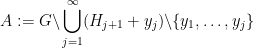
and ![{A := \bigcup_{j=1}^\infty [10^j, 1.1 \times 10^j]}](https://s0.wp.com/latex.php?latex=%7BA+%3A%3D+%5Cbigcup_%7Bj%3D1%7D%5E%5Cinfty+%5B10%5Ej%2C+1.1+%5Ctimes+10%5Ej%5D%7D&bg=ffffff&fg=000000&s=0&c=20201002) . Finally, the presence of the shift is also necessary, as can be seen by considering the example of being the odd numbers in
. Finally, the presence of the shift is also necessary, as can be seen by considering the example of being the odd numbers in  , though in the case
  one can of course delete the shift at the cost of giving up the containment .
Theorem 1 resembles other theorems in density Ramsey theory, such as Szemerédi’s theorem, but with the notable difference that the pattern located in the dense set 


The properties of being finite or infinite are neither closed nor open. Define a smallness property to be a closed (or compact) property of subsets of
-
elements.
-
elements, where
-
elements, where
is the
element of
-
halts when given
 an -large set.
Theorem 1 is then equivalent to the following “almost finitary” version (cf. this previous discussion of almost finitary versions of the infinite pigeonhole principle):
Theorem 2 (Almost finitary form of main theorem) Letbe a Følner sequence in
, and let
be a largeness property for each
such that if
is such that
for all
, then there exists a shift
Proof of Theorem 2 assuming Theorem 1. Let 


Proof of Theorem 1 assuming Theorem 2. Let 
Remark 3 Define a relationbetween
by declaring
if
is an open subset of
is also open. Indeed, if
, then
, and then any
that contains both
lies in
.

For each specific largeness property, such as the examples listed previously, Theorem 2 can be viewed as a finitary assertion (at least if the property is “computable” in some sense), but if one quantifies over all largeness properties, then the theorem becomes infinitary. In the spirit of the Paris-Harrington theorem, I would in fact expect some cases of Theorem 2 to undecidable statements of Peano arithmetic, although I do not have a rigorous proof of this assertion.
Despite the complicated finitary interpretation of this theorem, I was still interested in trying to write the proof of Theorem 1 in some sort of “pseudo-finitary” manner, in which one can see analogies with finitary arguments in additive combinatorics. The proof of Theorem 1 that I give below the fold is my attempt to achieve this, although to avoid a complete explosion of “epsilon management” I will still use at one juncture an ergodic theory reduction from the original paper of Kra et al. that relies on such infinitary tools as the ergodic decomposition, the ergodic theory, and the spectral theorem. Also some of the steps will be a little sketchy, and assume some familiarity with additive combinatorics tools (such as the arithmetic regularity lemma).
Tim Gowers, Ben Green, Freddie Manners, and I have just uploaded to the arXiv our paper “Marton’s conjecture in abelian groups with bounded torsion“. This paper fully resolves a conjecture of Katalin Marton (the bounded torsion case of the Polynomial Freiman–Ruzsa conjecture (first proposed by Katalin Marton):
Theorem 1 (Marton’s conjecture) Let
-torsion group (thus,
for all
), and let
. Then
translates of a subgroup
of
. Moreover,
for some
.
We had previously established the 


Our proof techniques are a modification of those in our previous paper, and in particular continue to be based on the theory of Shannon entropy. For inductive purposes, it turns out to be convenient to work with the following version of the conjecture (which, up to
Theorem 2 (Marton’s conjecture, entropy form) Let
be independent finitely supported random variables on
where
denotes Shannon entropy. Then there is a uniform random variable
on a subgroup
where
denotes the entropic Ruzsa distance (see previous blog post for a definition); furthermore, if all the
take values in some symmetric set
, then
for some
.
![\displaystyle {\bf H}[X_1+\dots+X_m] - \frac{1}{m} \sum_{i=1}^m {\bf H}[X_i] \leq \log K,](https://s0.wp.com/latex.php?latex=%5Cdisplaystyle+%7B%5Cbf+H%7D%5BX_1%2B%5Cdots%2BX_m%5D+-+%5Cfrac%7B1%7D%7Bm%7D+%5Csum_%7Bi%3D1%7D%5Em+%7B%5Cbf+H%7D%5BX_i%5D+%5Cleq+%5Clog+K%2C&bg=ffffff&fg=000000&s=0&c=20201002)
![\displaystyle \frac{1}{m} \sum_{i=1}^m d[X_i; U_H] \ll m^3 \log K,](https://s0.wp.com/latex.php?latex=%5Cdisplaystyle+%5Cfrac%7B1%7D%7Bm%7D+%5Csum_%7Bi%3D1%7D%5Em+d%5BX_i%3B+U_H%5D+%5Cll+m%5E3+%5Clog+K%2C&bg=ffffff&fg=000000&s=0&c=20201002)
As a first approximation, one should think of all the
The strategy, as with the previous paper, is to attempt an entropy decrement argument: to try to locate modifications 
![\displaystyle {\bf H}[X_1+\dots+X_m] - \frac{1}{m} \sum_{i=1}^m {\bf H}[X_i]](https://s0.wp.com/latex.php?latex=%5Cdisplaystyle+%7B%5Cbf+H%7D%5BX_1%2B%5Cdots%2BX_m%5D+-+%5Cfrac%7B1%7D%7Bm%7D+%5Csum_%7Bi%3D1%7D%5Em+%7B%5Cbf+H%7D%5BX_i%5D+&bg=ffffff&fg=000000&s=0&c=20201002)
which turns out to be a convenient metric for progress (for instance, this quantity is non-negative, and vanishes if and only if the 
As before, we search for such improved random variables 


Up until now, the argument does not use the 

In the endgame, the any pair of these three random variables are close to independent (after conditioning on the total sum
Besides the polynomial Bogolyubov conjecture mentioned above (which we do not know how to address by entropy methods), the other natural question is to try to develop a characteristic zero version of this theory in order to establish the polynomial Freiman–Ruzsa conjecture over torsion-free groups, which in our language asserts (roughly speaking) that random variables of small entropic doubling are close (in Ruzsa distance) to a discrete Gaussian random variable, with good bounds. The above machinery is consistent with this conjecture, in that it produces lots of independent variables related to the original variable, various linear combinations of which obey the same sort of entropy estimates that gaussian random variables would exhibit, but what we are missing is a way to get back from these entropy estimates to an assertion that the random variables really are close to Gaussian in some sense. In continuous settings, Gaussians are known to extremize the entropy for a given variance, and of course we have the central limit theorem that shows that averages of random variables typically converge to a Gaussian, but it is not clear how to adapt these phenomena to the discrete Gaussian setting (without the circular reasoning of assuming the polynoimal Freiman–Ruzsa conjecture to begin with).
Earlier this year, I gave a series of lectures at the Joint Mathematics Meetings at San Francisco. I am uploading here the slides for these talks:
- “Machine assisted proof” (Video here)
- “Translational tilings of Euclidean space” (Video here)
- “Correlations of multiplicative functions” (Video here)
I also have written a text version of the first talk, which has been submitted to the Notices of the American Mathematical Society.
Since the release of my preprint with Tim, Ben, and Freddie proving the Polynomial Freiman-Ruzsa (PFR) conjecture over 
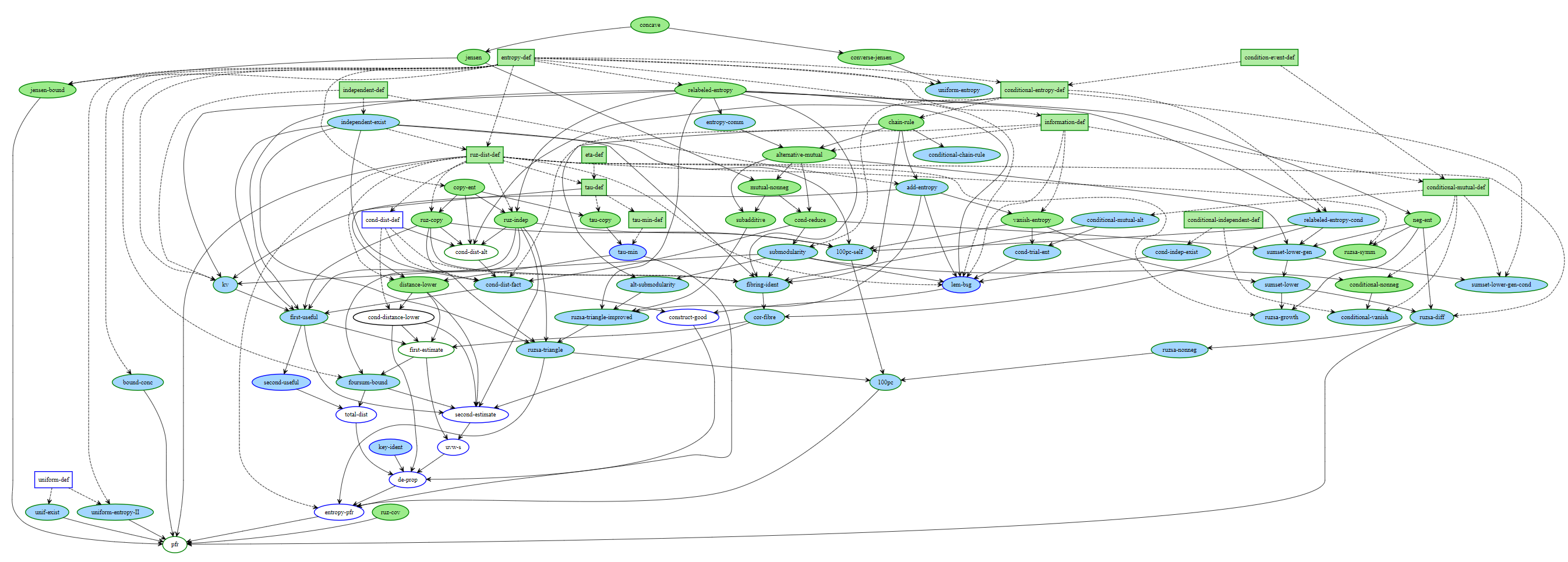
The color coding of the various bubbles (for lemmas) and rectangles (for definitions) is explained in the legend to the dependency graph, but roughly speaking the green bubbles/rectangles represent lemmas or definitions that have been fully formalized, and the blue ones represent lemmas or definitions which are ready to be formalized (their statements, but not proofs, have already been formalized, as well as those of all prerequisite lemmas and proofs). The goal is to get all the bubbles leading up to and including the “pfr” bubble at the bottom colored in green.
In this post I would like to give a quick “tour” of the project, to give a sense of how it operates. If one clicks on the “pfr” bubble at the bottom of the dependency graph, we get the following:

Here, Blueprint is displaying a human-readable form of the PFR statement. This is coming from the corresponding portion of the blueprint, which also comes with a human-readable proof of this statement that relies on other statements in the project:

(I have cropped out the second half of the proof here, as it is not relevant to the discussion.)
Observe that the “pfr” bubble is white, but has a green border. This means that the statement of PFR has been formalized in Lean, but not the proof; and the proof itself is not ready to be formalized, because some of the prerequisites (in particular, “entropy-pfr” (Theorem 6.16)) do not even have their statements formalized yet. If we click on the “Lean” link below the description of PFR in the dependency graph, we are lead to the (auto-generated) Lean documentation for this assertion:

This is what a typical theorem in Lean looks like (after a procedure known as “pretty printing”). There are a number of hypotheses stated before the colon, for instance that 


The astute reader may notice that the above theorem seems to be missing one or two details, for instance it does not explicitly assert that

Here we see that
Filling in this “sorry” is too hard to do right now, so let’s look for a simpler task to accomplish instead. Here is a simple intermediate lemma “ruzsa-nonneg” that shows up in the proof:

The expression ![d[X; Y]](https://s0.wp.com/latex.php?latex=d%5BX%3B+Y%5D&bg=ffffff&fg=545454&s=0&c=20201002)


“ruzsa-diff” is also blue and bordered in green, so it has the same current status as “ruzsa-nonneg“: the statement is formalized, and the proof is ready to be formalized also, but the proof has not been written in Lean yet. The quantity ![H[X]](https://s0.wp.com/latex.php?latex=H%5BX%5D&bg=ffffff&fg=545454&s=0&c=20201002)
Looking at Lemma 3.11 and Lemma 3.13 it is clear how the former will imply the latter: the quantity ![|H[X] - H[Y]|](https://s0.wp.com/latex.php?latex=%7CH%5BX%5D+-+H%5BY%5D%7C&bg=ffffff&fg=545454&s=0&c=20201002)

Again we have a “sorry” to indicate that this lemma does not currently have a proof. The Lean notation (as well as the name of the lemma) differs a little from the LaTeX version for technical reasons that we will not go into here. (Also, the variables 

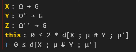
OK, I’m now going to try to fill in the latter “sorry”. In my local copy of the PFR github repository, I open up the relevant Lean file in my editor (Visual Studio Code, with the lean4 extension) and navigate to the “sorry” of “rdist_nonneg”. The accompanying “Lean infoview” then shows the current state of the Lean proof:

Here we see a number of ambient hypotheses (e.g., that 
OK, so now I’ll try to prove the claim. This is accomplished by applying a series of “tactics” to transform the goal and/or hypotheses. The first step I’ll do is to put in the factor of

I now have two goals (and two “sorries”): one to show that ![0 \leq 2 d[X;Y]](https://s0.wp.com/latex.php?latex=0+%5Cleq+2+d%5BX%3BY%5D&bg=ffffff&fg=545454&s=0&c=20201002)
![0 \leq d[X,Y]](https://s0.wp.com/latex.php?latex=0+%5Cleq+d%5BX%2CY%5D&bg=ffffff&fg=545454&s=0&c=20201002)
Let’s fill in the first “sorry”. The tactic state now looks like this (cropping out some irrelevant hypotheses):
Here I can use a handy tactic “linarith“, which solves any goal that can be derived by linear arithmetic from existing hypotheses:

This works, and now the tactic state reports no goals left to prove on this branch, so we move on to the remaining sorry, in which the goal is now to prove

Here we will try to invoke Lemma 3.11. I add the following lines of code:

The Lean tactic “have” roughly corresponds to the Mathematical English phrase “We have the statement…” or “We claim the statement…”; like “suffices”, it splits a goal into two subgoals, though in the reversed order to “suffices”.
I again have two subgoals, one to prove the bound ![|H[X]-H[Y]| \leq 2 d[X;Y]](https://s0.wp.com/latex.php?latex=%7CH%5BX%5D-H%5BY%5D%7C+%5Cleq+2+d%5BX%3BY%5D&bg=ffffff&fg=545454&s=0&c=20201002)


So I try this (by clicking on the suggested code, which automatically pastes it into the right location), and it works, leaving me with the final “sorry”:

The lean tactic “exact” corresponds, roughly speaking, to the Mathematical English phrase “But this is exactly …”.
At this point I should mention that I also have the Github Copilot extension to Visual Studio Code installed. This is an AI which acts as an advanced autocomplete that can suggest possible lines of code as one types. In this case, it offered a suggestion which was almost correct (the second line is what we need, whereas the first is not necessary, and in fact does not even compile in Lean):

In any event, “exact?” worked in this case, so I can ignore the suggestion of Copilot this time (it has been very useful in other cases though). I apply the “exact?” tactic a second time and follow its suggestion to establish the matching bound ![0 \leq |H[X] - H[Y]|](https://s0.wp.com/latex.php?latex=0+%5Cleq+%7CH%5BX%5D+-+H%5BY%5D%7C&bg=ffffff&fg=545454&s=0&c=20201002)

(One can find documention for the “abs_nonneg” method here. Copilot, by the way, was also able to resolve this step, albeit with a slightly different syntax; there are also several other search engines available to locate this method as well, such as Moogle. One of the main purposes of the Lean naming conventions for lemmas, by the way, is to facilitate the location of methods such as “abs_nonneg”, which is easier figure out how to search for than a method named (say) “Lemma 1.2.1”.) To fill in the final “sorry”, I try “exact?” one last time, to figure out how to combine 

Note that all the squiggly underlines have disappeared, indicating that Lean has accepted this as a valid proof. The documentation for “ge_trans” may be found here. The reader may observe that this method uses the 


It is possible to compactify this proof quite a bit by cutting out several intermediate steps (a procedure sometimes known as “code golf“):

And now the proof is done! In the end, it was literally a “one-line proof”, which makes sense given how close Lemma 3.11 and Lemma 3.13 were to each other.
The current version of Blueprint does not automatically verify the proof (even though it does compile in Lean), so we have to manually update the blueprint as well. The LaTeX for Lemma 3.13 currently looks like this:

I add the “\leanok” macro to the proof, to flag that the proof has now been formalized:

I then push everything back up to the master Github repository. The blueprint will take quite some time (about half an hour) to rebuild, but eventually it does, and the dependency graph (which Blueprint has for some reason decided to rearrange a bit) now shows “ruzsa-nonneg” in green:

And so the formalization of PFR moves a little bit closer to completion. (Of course, this was a particularly easy lemma to formalize, that I chose to illustrate the process; one can imagine that most other lemmas will take a bit more work.) Note that while “ruzsa-nonneg” is now colored in green, we don’t yet have a full proof of this result, because the lemma “ruzsa-diff” that it relies on is not green. Nevertheless, the proof is locally complete at this point; hopefully at some point in the future, the predecessor results will also be locally proven, at which point this result will be completely proven. Note how this blueprint structure allows one to work on different parts of the proof asynchronously; it is not necessary to wait for earlier stages of the argument to be fully formalized to start working on later stages, although I anticipate a small amount of interaction between different components as we iron out any bugs or slight inaccuracies in the blueprint. (For instance, I am suspecting that we may need to add some measurability hypotheses on the random variables 
That concludes the brief tour! If you are interested in learning more about the project, you can follow the Zulip chat stream; you can also download Lean and work on the PFR project yourself, using a local copy of the Github repository and sending pull requests to the master copy if you have managed to fill in one or more of the “sorry”s in the current version (but if you plan to work on anything more large scale than filling in a small lemma, it is good to announce your intention on the Zulip chat to avoid duplication of effort) . (One key advantage of working with a project based around a proof assistant language such as Lean is that it makes large-scale mathematical collaboration possible without necessarily having a pre-established level of trust amongst the collaborators; my fellow repository maintainers and I have already approved several pull requests from contributors that had not previously met, as the code was verified to be correct and we could see that it advanced the project. Conversely, as the above example should hopefully demonstrate, it is possible for a contributor to work on one small corner of the project without necessarily needing to understand all the mathematics that goes into the project as a whole.)
If one just wants to experiment with Lean without going to the effort of downloading it, you can playing try the “Natural Number Game” for a gentle introduction to the language, or the Lean4 playground for an online Lean server. Further resources to learn Lean4 may be found here.
Tim Gowers, Ben Green, Freddie Manners, and I have just uploaded to the arXiv our paper “On a conjecture of Marton“. This paper establishes a version of the notorious Polynomial Freiman–Ruzsa conjecture (first proposed by Katalin Marton):
Theorem 1 (Polynomial Freiman–Ruzsa conjecture) Letbe such that
translates of a subspace
of cardinality at most
The previous best known result towards this conjecture was by Konyagin (as communicated in this paper of Sanders), who obtained a similar result but with 


The exponent 
In this paper we will focus exclusively on the characteristic
Much of the prior progress on this sort of result has proceeded via Fourier analysis. Perhaps surprisingly, our approach uses no Fourier analysis whatsoever, being conducted instead entirely in “physical space”. Broadly speaking, it follows a natural strategy, which is to induct on the doubling constant 


 to means that the various Ruzsa distances that need to be summed are controlled by a convergent geometric series).
There are a number of possible ways to try to “improve” a set
- (i) Replacing
) of a large subspace
- (ii) Replacing
for a “typical”
. For instance, if
Unfortunately, there are sets 

This begins to suggest a potential strategy: show that at least one of the operations (i) or (ii) will improve the doubling constant, or at least not worsen it too much; and in the latter case, perform some more complicated operation to locate the desired doubling constant improvement.
A sign that this strategy might have a chance of working is provided by the following heuristic argument. If 


Unfortunately, this argument does not seem to be easily made rigorous using the traditional doubling constant; even the significantly weaker statement that 


 is defined as


Applying this inequality with 


 is determined by
  once one fixes
  )
) 
 , then at least one of
  or
or  will be less than or equal to
  . This is the entropy analogue of at least one of (i) or (ii) improving, or at least not degrading the doubling constant, although there are some minor technicalities involving how one deals with the conditioning to in the second term that we will gloss over here (one can pigeonhole the instances of to different events
  ,
,  , and “depolarise” the induction hypothesis to deal with distances
  between pairs of random variables that do not necessarily have the same distribution). Furthermore, we can even calculate the defect in the above inequality: a careful inspection of the above argument eventually reveals that

 . This leads (modulo some technicalities) to the following interesting conclusion: if neither (i) nor (ii) leads to an improvement in the entropic doubling constant, then and
  are conditionally independent relative to
  . This situation (or an approximation to this situation) is what we refer to in the paper as the “endgame”.
A version of this endgame conclusion is in fact valid in any characteristic. But in characteristic
 , and using symmetry we now conclude that if we are in the endgame exactly (so that the mutual information is zero), then the independent sum of two copies of
  has exactly the same distribution; in particular, the entropic doubling constant here is zero, which is certainly a reduction in the doubling constant.
To deal with the situation where the conditional mutual information is small but not completely zero, we have to use an entropic version of the Balog-Szemeredi-Gowers lemma, but fortunately this was already worked out in an old paper of mine (although in order to optimise the final constant, we ended up using a slight variant of that lemma).
I am planning to formalize this paper in the Lean4 language. Further discussion of this project will take place on this Zulip stream, and the project itself will be held at this Github repository.
Rachel Greenfeld and I have just uploaded to the arXiv our paper “Undecidability of translational monotilings“. This is a sequel to our previous paper in which we constructed a translational monotiling 


One of the motivations of this conjecture was the observation of Hao Wang that if the periodic tiling conjecture were true, then the translational monotiling problem is (algorithmically) decidable: there is a Turing machine which, when given a dimension
On the other hand, Wang’s argument is not known to be reversible: the failure of the periodic tiling conjecture does not automatically imply the undecidability of the translational monotiling problem, as it does not rule out the existence of some other algorithm to determine tiling that does not rely on the existence of a periodic tiling. (For instance, even with the newly discovered hat and spectre tiles, it remains an open question whether the isometric monotiling problem for (say) polygons with rational coefficients in
The main result of this paper settles this question (with one caveat):
Theorem 1 There does not exist any algorithm which, given a dimension
of
of
The caveat is that we have to work with periodic subsets 

Because of a well known link between algorithmic undecidability and logical undecidability (also known as logical independence), the main theorem also implies the existence of an (in principle explicitly describable) dimension
As a consequence of our method, we can also replace 
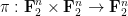
We now describe some of the main ideas of the proof. It is a common technique to show that a given problem is undecidable by demonstrating that some other problem that was already known to be undecidable can be “encoded” within the original problem, so that any algorithm for deciding the original problem would also decide the embedded problem. Accordingly, we will encode the Wang tiling problem as a monotiling problem in
Problem 2 (Wang tiling problem) Given a finite collection
of Wang tiles (unit squares with each side assigned some color from a finite palette), is it possible to tile the plane with translates of these tiles along the standard lattice
, such that adjacent tiles have matching colors along their common edge?
It is a famous result of Berger that this problem is undecidable. The embedding of this problem into the higher-dimensional translational monotiling problem proceeds through some intermediate problems. Firstly, it is an easy matter to embed the Wang tiling problem into a similar problem which we call the domino problem:
Problem 3 (Domino problem) Given a finite collection
(resp.
) of horizontal (resp. vertical) dominoes – pairs of adjacent unit squares, each of which is decorated with an element of a finite set
Indeed, one just has to interpet each Wang tile as a separate “pip”, and define the domino sets
Next, we embed the domino problem into a Sudoku problem:
Problem 4 (Sudoku problem) Given a column width
, a collection
of functions
, and an “initial condition”
(which we will not detail here, as it is a little technical), is it possible to assign a digit
to each cell
in the “Sudoku board”
such that for any slope
and intercept
, the digits
along the line
lie in
The most novel part of the paper is the demonstration that the domino problem can indeed be embedded into the Sudoku problem. The embedding of the Sudoku problem into the monotiling problem follows from a modification of the methods in our previous papers, which had also introduced versions of the Sudoku problem, and created a “tiling language” which could be used to “program” various problems, including the Sudoku problem, as monotiling problems.
To encode the domino problem into the Sudoku problem, we need to take a domino function 


and a typical instance of the final component 

Amusingly, the decoration here is essentially following the rules of the children’s game “Fizz buzz“.
To demonstrate the embedding, we thus need to produce a specific Sudoku rule 


Ben Green, Freddie Manners and I have just uploaded to the arXiv our preprint “Sumsets and entropy revisited“. This paper uses entropy methods to attack the Polynomial Freiman-Ruzsa (PFR) conjecture, which we study in the following two forms:
Conjecture 1 (Weak PFR over) Let
be a finite non-empty set whose doubling constant
is at most
that has affine dimension
Conjecture 2 (PFR over) Let
be a non-empty set whose doubling constant
is at most
cosets of a subspace of cardinality at most
Our main results are then as follows.
Theorem 3 If, then
- (i) There is a subset
- (ii) There is a subset
of affine dimension
goes to zero as
).
- (iii) If Conjecture 2 holds, then there is a subset
The skew-dimension of a set is a quantity smaller than the affine dimension which is defined recursively; the precise definition is given in the paper, but suffice to say that singleton sets have dimension 


Part (i) of this theorem was implicitly proven by Pálvölgi and Zhelezov by a different method. Part (ii) with 
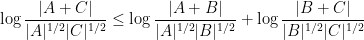
Our proof strategy is to establish these combinatorial additive combinatorics results by using entropic additive combinatorics, in which we replace sets
For instance, the analogue of the combinatorial doubling constant
![\displaystyle \sigma_{\mathrm{ent}}[X] := {\exp( \bf H}(X_1+X_2) - {\bf H}(X) )](https://s0.wp.com/latex.php?latex=%5Cdisplaystyle++%5Csigma_%7B%5Cmathrm%7Bent%7D%7D%5BX%5D+%3A%3D+%7B%5Cexp%28+%5Cbf+H%7D%28X_1%2BX_2%29+-+%7B%5Cbf+H%7D%28X%29+%29&bg=ffffff&fg=000000&s=0&c=20201002) in , where are independent copies of and denotes Shannon entropy. There is also an analogue of the Ruzsa distance
in , where are independent copies of and denotes Shannon entropy. There is also an analogue of the Ruzsa distance 
 of , namely the entropic Ruzsa distance
 are independent copies of respectively. (Actually, one thing we show in our paper is that the independence hypothesis can be dropped, and this only affects the entropic Ruzsa distance by a factor of three at worst.) Many of the results about sumsets and Ruzsa distance have entropic analogues, but the entropic versions are slightly better behaved; for instance, we have a contraction property
 is a homomorphism. In fact we have a refinement of this inequality in which the gap between these two quantities can be used to control the entropic distance between “fibers” of (in which one conditions
  and
and  to be fixed). On the other hand, there are direct connections between the combinatorial and entropic sumset quantities. For instance, if
  is a random variable drawn uniformly from , then
 ![\displaystyle \sigma_{\mathrm{ent}}[U_A] \leq \sigma[A].](https://s0.wp.com/latex.php?latex=%5Cdisplaystyle++%5Csigma_%7B%5Cmathrm%7Bent%7D%7D%5BU_A%5D+%5Cleq+%5Csigma%5BA%5D.&bg=ffffff&fg=000000&s=0&c=20201002) has small doubling, then has small entropic doubling. In the converse direction, if has small entropic doubling, then is close (in entropic Ruzsa distance) to a uniform random variable
has small doubling, then has small entropic doubling. In the converse direction, if has small entropic doubling, then is close (in entropic Ruzsa distance) to a uniform random variable  drawn from a set of small doubling; a version of this statement was proven in an old paper of myself, but we establish here a quantitatively efficient version, established by rewriting the entropic Ruzsa distance in terms of certain Kullback-Liebler divergences.
Our first main result is a “99% inverse theorem” for entropic Ruzsa distance: if 

We now sketch how these tools are used to prove our main theorem. For (i), we reduce matters to establishing the following bilinear entropic analogue: given two non-empty finite subsets 


 have skew-dimension at most
  , for some absolute constant . This can be shown by an induction on
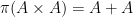
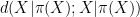
  (say). One applies a non-trivial coordinate projection
  to . If
  and
and  are very close in entropic Ruzsa distance, then the 99% inverse theorem shows that these random variables must each concentrate at a point (because
  has no non-trivial finite subgroups), and can pass to a fiber of these points and use the induction hypothesis. If instead and are far apart, then by the behavior of entropy under projections one can show that the fibers of and under are closer on average in entropic Ruzsa distance of and themselves, and one can again proceed using the induction hypothesis.
For parts (ii) and (iii), we first use an entropic version of an observation of Manners that sets of small doubling in
 take values in a torsion-free abelian group such as ; this turns out to follow from two applications of the entropy submodularity inequality. One corollary of this (and the behavior of entropy under projections) is that
  and
and  worlds that is used to prove (ii), (iii): while (iii) relies on the still unproven PFR conjecture over , (ii) uses the unconditional progress on PFR by Konyagin, as detailed in this survey of Sanders. The argument has a similar inductive structure to that used to establish (i) (and if one is willing to replace by then the argument is in fact relatively straightforward and does not need any deep partial results on the PFR).
As one byproduct of our analysis we also obtain an appealing entropic reformulation of Conjecture 2, namely that if
![\displaystyle d_{\mathrm{ent}}(X, U_H) \ll \sigma_{\mathrm{ent}}[X].](https://s0.wp.com/latex.php?latex=%5Cdisplaystyle++d_%7B%5Cmathrm%7Bent%7D%7D%28X%2C+U_H%29+%5Cll+%5Csigma_%7B%5Cmathrm%7Bent%7D%7D%5BX%5D.&bg=ffffff&fg=000000&s=0&c=20201002)
![\displaystyle d_{\mathrm{ent}}(X, U_H) \ll_\varepsilon \sigma_{\mathrm{ent}}[X] + \sigma_{\mathrm{ent}}^{3+\varepsilon}[X]](https://s0.wp.com/latex.php?latex=%5Cdisplaystyle++d_%7B%5Cmathrm%7Bent%7D%7D%28X%2C+U_H%29+%5Cll_%5Cvarepsilon+%5Csigma_%7B%5Cmathrm%7Bent%7D%7D%5BX%5D+%2B+%5Csigma_%7B%5Cmathrm%7Bent%7D%7D%5E%7B3%2B%5Cvarepsilon%7D%5BX%5D&bg=ffffff&fg=000000&s=0&c=20201002)
 , by using Konyagin’s partial result towards the PFR.
Hariharan Narayanan, Scott Sheffield, and I have just uploaded to the arXiv our paper “Sums of GUE matrices and concentration of hives from correlation decay of eigengaps“. This is a personally satisfying paper for me, as it connects the work I did as a graduate student (with Allen Knutson and Chris Woodward) on sums of Hermitian matrices, with more recent work I did (with Van Vu) on random matrix theory, as well as several other results by other authors scattered across various mathematical subfields.
Suppose 


One of my favourite open problems is to come up with a theory of “free hives” that allows one to explain the latter fact from the former. This is still unresolved, but we are now beginning to make a bit of progress towards this goal. We know (for instance from the calculations of Coquereaux and Zuber) that if 
In this paper, we are able to accomplish the first half of this goal, assuming that the spectra 


Augmented hives seem tricky to work with directly, but by adapting the octahedron recurrence introduced for this problem by Knutson, Woodward, and myself some time ago (which is related to the associativity 
On the other hand, the piecewise linear map, initially defined by iterating the octahedron relation 
It would be more convenient to study the concentration of each linear map separately, rather than their supremum. By the Cheeger inequality, it turns out that one can relate the latter to the former provided that one has good control on the Cheeger constant of the underlying measure on the Gelfand-Tsetlin cones. Fortunately, the measure is log-concave, so one can use the very recent work of Klartag on the KLS conjecture to eliminate the supremum (up to a logarithmic loss which is only moderately annoying to deal with).
It remains to obtain concentration on the linear map associated to a given lozenge tiling. After stripping away some contributions coming from lozenges near the edge (using some eigenvalue rigidity results of Van Vu and myself), one is left with some bulk contributions which ultimately involve eigenvalue interlacing gaps such as

 is the
  eigenvalue of the top left
  minor of , and
  is in the bulk region
  for some fixed . To get the desired result, one needs some non-trivial correlation decay in for these statistics. If one was working with eigenvalue gaps
  rather than interlacing results, then such correlation decay was conveniently obtained for us by recent work of Cippoloni, Erdös, and Schröder. So the last remaining challenge is to understand the relation between eigenvalue gaps and interlacing gaps.
For this we turned to the work of Metcalfe, who uncovered a determinantal process structure to this problem, with a kernel associated to Lagrange interpolation polynomials. It is possible to satisfactorily estimate various integrals of these kernels using the residue theorem and eigenvalue rigidity estimates, thus completing the required analysis.
Asgar Jamneshan, Or Shalom, and myself have just uploaded to the arXiv our preprints “A Host–Kra 


Recent Comments