
These lecture notes are a continuation of the 254A lecture notes from the previous quarter.
We consider the Euler equations for incompressible fluid flow on a Euclidean space 


In Eulerian coordinates, the Euler equations read


where 


We will refer to the coordinates
In view of this, it is natural to ask whether there is an alternate way to formulate the continuum limit of incompressible inviscid fluids, by using a continuous version 


Given a smooth and bounded velocity field 

in view of (2), this describes the trajectory (in 
for 

Despite the popularity of the initial condition (4), we will try to keep conceptually separate the Eulerian space 
Exercise 1 Let
- If
is a smooth map, show that there exists a unique smooth trajectory map
for all
- Show that if
is a diffeomorphism and
is also a diffeomorphism.
Remark 2 The first of the Euler equations (1) can now be written in the form
which can be viewed as a continuous limit of Newton’s first law
.
Call a diffeomorphism 
for all 


for all 


The divergence-free condition 

Lemma 3 Let
is volume-preserving for all
Proof: Since 

for all
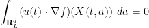
for all
which by integration by parts gives

for all
To prove the converse implication, it is convenient to introduce the labels map 

for all 

where 
acting on functions on

for any test function 

and hence

for any 
Thus 

Exercise 4 Let
be a continuously differentiable map from the time interval
to the general linear group
of invertible
and use this and (6) to give an alternate proof of Lemma 3 that does not involve any integration in space.

Remark 5 One can view the use of Lagrangian coordinates as an extension of the method of characteristics. Indeed, from the chain rule we see that for any smooth function
of Eulerian spacetime, one has
and hence any transport equation that in Eulerian coordinates takes the form
for smooth functions
of Eulerian spacetime is equivalent to the ODE
where
are the smooth functions of Lagrangian spacetime defined by


In this set of notes we recall some basic differential geometry notation, particularly with regards to pullbacks and Lie derivatives of differential forms and other tensor fields on manifolds such as
Remark 6 One can also write the Navier-Stokes equations in Lagrangian coordinates, but the equations are not expressed in a favourable form in these coordinates, as the Laplacian
appearing in the viscosity term becomes replaced with a time-varying Laplace-Beltrami operator. As such, we will not discuss the Lagrangian coordinate formulation of Navier-Stokes here.
— 1. Pullbacks and Lie derivatives —
In order to efficiently change coordinates, it is convenient to use the language of differential geometry, which is designed to be almost entirely independent of the choice of coordinates. We therefore spend some time recalling the basic concepts of differential geometry that we will need. Our presentation will be based on explicitly working in coordinates; there are of course more coordinate-free approaches to the subject (for instance setting up the machinery of vector bundles, or of derivations), but we will not adopt these approaches here.
Throughout this section, we fix a diffeomorphism 


These operations are all compatible with each other in various ways; for instance, if 

-
if and only if
.
-
if and only if
.
- The map
is an isomorphism of
-algebras.
- The map
is an algebra isomorphism.
Differential forms. The next family of structures we will pull back are that of differential forms, which we will define using coordinates. (See also my previous notes on this topic for more discussion on differential forms.) For any 


- A
-form is just a scalar field
;
- A
-form, when viewed in coordinates, is a collection
of
- A
-form, when viewed in coordinates, is a collection
of
scalar functions with
(so in particular
);
- A
-form, when viewed in coordinates, is a collection
of
scalar functions with
,
, and
.
The antisymmetry makes the component 


If 


More generally, given two forms 


where 


Exercise 7 Show that the wedge product is a bilinear map from
to
that obeys the supercommutative property
for
for
. (In other words, the space of formal linear combinations of forms, graded by the parity of the order of the forms, is a supercommutative algebra. Very roughly speaking, the prefix “super” means that “odd order objects anticommute with each other rather than commute”.)


If 

It is easy to verify that this is indeed a 
- If
.
- If
is a continuously differentiable
.
- If
.
Exercise 8 If
and if


Each of the coordinates 


for any
One can of course define differential forms on Lagrangian space 


If 

with the usual summation conventions. Thus for instance
- If
is given by the same formula
as before.
- If
is given by the formula
.
- If
is given by the formula

It is easy to see that pullback 

Exercise 9 Let
. Show that
and if


One can integrate 


with the usual summation conventions. It can be shown that this definition is independent of the choice of parameterisation. For a more general manifold 


linking integration on differential forms with the Lebesgue (or Riemann) integral. We also record Stokes’ theorem

whenever 


From the change of variables formula we see that pullback also respects integration on manifolds, in that

whenever
Exercise 10 Establish the identity
Conclude in particular that


Vector fields. Having pulled back differential forms, we now pull back vector fields. A vector field 


where we multiply scalar functions against vector fields in the obvious fashion; compare this with the expansion 

The pullback 


for all 


with 

From the inverse function theorem one can also write

thus 
If 

Thus for instance if 
It is clear that 


or equivalently that

for 

If 


The contraction 


This can easily be seen to be a bijection between vector fields and 
In a similar spirit, the Hodge dual of a scalar field

and conversely the Hodge dual of a volume form is a scalar field:

More generally one can form a Hodge duality relationship between 


These operations behave well under pullback (if one assumes volume preservation in the case of the Hodge star):
Exercise 11
- (i) If
- (ii) If
- (iii) If
whenever
is a scalar field, vector field,


Exercise 12 (Cauchy-Binet formula) Let
be vector fields. Establish (a special case of) the Cauchy-Binet formula

Riemannian metrics. A Riemannian metric 


where 


this is a symmetric bilinear form in 
We can define the pullback metric 

this is easily seen to be a Riemannian metric on

for all

then we have the expected relationship
Exercise 13 If
is a diffeomorphism, show that
for any
for any
for any Riemannian metric


Exercise 14 Show that
.
Every Riemannian metric 


and similarly if 


These operations clearly invert each other: 


The musical isomorphism interacts well with pullback, provided that one also pulls back the metric
Exercise 15 If
for all
for all


We can now interpret some classical operations on vector fields in this differential geometry notation. For instance, if 

and also

and for 


Exercise 16 Formulate a definition for the pullback
of a rank
tensor field
for
) that generalises the pullback of differential forms, vector fields, and Riemannian metrics. Argue why your definition is the natural one.
Lie derivatives. Let 


with the convention that 
- If
is just the directional derivative of
.
- If
is the
- If
is the


One can interpret the Lie derivative as the infinitesimal version of pullback:
Exercise 17 Let
can be viewed as a smooth vector field on
More generally, if
is a smooth
where
denotes the material Lie derivative


Note that the material Lie derivative specialises to the material derivative when applied to scalar fields. The above exercise shows that the trajectory map intertwines the ordinary time derivative 
Remark 18 If one lets
be the trajectory map associated to a time-independent vector field
and
, then the above exercise shows that
for any differential form
(and has the advantage of readily extending to other tensors than differential forms, for which the Cartan formula is not available).
The Lie derivative behaves very well with respect to exterior product and exterior derivative:
Exercise 19 Let
also be continuously differentiable. Establish the Leibniz rule
If
of exterior derivative and Lie derivative.

Exercise 20 Let
where
is the divergence of
Exercise 21 Let
Conclude in particular that if
for any
.


The Lie derivative 


and the Lie derivative 


Thus for instance the Lie derivative of the Euclidean metric

(compare with the deformation tensor used in Notes 0).
We have similar properties to Exercise 19:
Exercise 22 Let
- (i) If
are continuously differentiable, establish the Leibniz rule
If
, establish the variant Leibniz rule
- (ii) If
are continuously differentiable, establish the Leibniz rule
similarly, for
- (iii) Establish the analogue of Exercise 17 in which the differential form
or a rank
- (iv) If
whenever


Exercise 23 If
whenever
is a continuously differentiable differential form, vector field, or metric tensor.

Exercise 24 If
are smooth, define the Lie bracket
by the formula
Establish the anti-symmetry
(so in particular
) and the Jacobi identity
and also
whenever
are smooth, and
![\displaystyle [Z,W] := {\mathcal L}_Z W.](https://s0.wp.com/latex.php?latex=%5Cdisplaystyle++%5BZ%2CW%5D+%3A%3D+%7B%5Cmathcal+L%7D_Z+W.&bg=ffffff&fg=000000&s=0&c=20201002)
![\displaystyle [[Z_1,Z_2],Z_3] + [[Z_2,Z_3],Z_1] + [[Z_3,Z_1],Z_2] = 0,](https://s0.wp.com/latex.php?latex=%5Cdisplaystyle++%5B%5BZ_1%2CZ_2%5D%2CZ_3%5D+%2B+%5B%5BZ_2%2CZ_3%5D%2CZ_1%5D+%2B+%5B%5BZ_3%2CZ_1%5D%2CZ_2%5D+%3D+0%2C&bg=ffffff&fg=000000&s=0&c=20201002)
![\displaystyle {\mathcal L}_{[Z,W]} \phi = {\mathcal L}_Z {\mathcal L}_W \phi - {\mathcal L}_W {\mathcal L}_Z \phi](https://s0.wp.com/latex.php?latex=%5Cdisplaystyle++%7B%5Cmathcal+L%7D_%7B%5BZ%2CW%5D%7D+%5Cphi+%3D+%7B%5Cmathcal+L%7D_Z+%7B%5Cmathcal+L%7D_W+%5Cphi+-+%7B%5Cmathcal+L%7D_W+%7B%5Cmathcal+L%7D_Z+%5Cphi&bg=ffffff&fg=000000&s=0&c=20201002)
Exercise 25 Formulate a definition for the Lie derivative
of a (continuously differentiable) rank
— 2. The Euler equations in differential geometry notation —
Now we write the Euler equations (1) in differential geometry language developed in the above section. This will make it relatively painless to change coordinates. As in the rest of this set of notes, we work formally, assuming that all fields are smooth enough to justify the manipulations below.
The Euler equations involve a time-dependent scalar field 


or equivalently (by Exercise 20 and the definition of material Lie derivative 

For the first equation, it is convenient to work instead with the covelocity field 
In coordinates, we have 

The left-hand side is close to the 


and so the first Euler equation becomes
Since 


We thus see that the Euler equations can be transformed to the system


Using the Cartan formula (19), one can also write (22) as

where 

In coordinates, (25) becomes

One advantage of the formulation (22)–(24) is that one can pull back by an arbitrary diffeomorphic change of coordinates (both time-dependent and time-independent), with the only things potentially changing being the material Lie derivative
For instance, suppose 


Strictly speaking, this is not a diffeomorphism due to singularities at 


thus the pullback metric 


The volume form 

If (by slight abuse of notation) we write the components of 


and the third equation (24) is
which by the product rule and Exercise 20 becomes
or after expanding in coordinates

If one substitutes (27) into (26) in the


One should compare how readily one can derive these equations using the differential geometry formalism with the more pedestrian aproach using the chain rule:
Exercise 26 Starting with a smooth solution
to the Euler equations (1) in
, and transforming to cylindrical coordinates
, establish the chain rule formulae
and use this and the identity
to rederive the system (28)–(31) (away from the


Exercise 27 Turkington coordinates
are a variant of cylindrical coordinates
, defined by the formulae
the advantage of these coordinates are that the map from Cartesian coordinates
to Turkington coordinates
is volume preserving. Show that in these coordinates, the Euler equations become
(These coordinates are particularly useful for studying solutions to Euler that are “axisymmetric with swirl”, in the sense that the fields
do not depend on the
variable, so that all the terms involving
vanish; one can specialise further to the case of solutions that are “axisymmetric without swirl”, in which case
also vanishes.)


We can use the differential geometry formalism to formally verify the conservation laws of the Euler equation. We begin with conservation of energy
Formally differentiating this in time (and noting that the form 


Using (22), we can write

From the Cartan formula (19) one has 


From Exercise 21 we thus formally obtain the conservation law 
Now suppose that

Taking traces in (21), this implies in particular that

(Geometrically, this implication arises because the volume form

As

Using (22), the left-hand side is

By Cartan’s formula, 


By Exercise 24, we have 


and so this integral also vanishes. Thus we obtain the conservation law 

for 

for 
Exercise 28 Let
. (Hint: use (21) to show that all the second derivatives of components of
The vorticity 

It already made an appearance in Notes 3 from the previous quarter. Taking exterior derivatives of (22) using (10) and Exercise 19 we obtain the appealingly simple vorticity equation

In two and three dimensions we may take the Hodge dual 

In two dimensions, this gives us a lot of conservation laws, since one can apply the scalar chain rule to then formally conclude that

for any 


for any such function 


In three dimensions there is also an interesting conservation law involving the vorticity. Observe that the wedge product 


is a formally conserved quantity of the Euler equations. Indeed, formally differentiating and using Exercise 21 we have
From the Leibniz rule and (32) we have

Applying (22) we can write this expression as 


Exercise 29 Formally verify the conservation of momentum, angular momentum, and helicity directly from the original form (1) of the Euler equations.
Exercise 30 In even dimensions
, show that the integral
(formed by taking the exterior product of
copies of
, show that the generalised helicity
is conserved by the flow. (This observation is due to Denis Serre, as well as unpublished work of Tartar.)
As it turns out, there are no further conservation laws for the Euler equations in Eulerian coordinates that are linear or quadratic integrals of the velocity field and its derivatives, at least in three dimensions; see this paper of Denis Serre. In particular, the Euler equations are not believed to be completely integrable. (But there are a few more conserved integrals of motion in the Lagrangian formalism; see Exercise 41.)
Exercise 31 Let
be a smooth solution to the Euler equations in three dimensions
be an arbitrary smooth scalar field. Establish Ertel’s theorem

Exercise 32 (Clebsch variables) Let
takes the form
for some smooth scalar fields
.
- (i) Show that at all subsequent times
where
are smooth scalar fields obeying the transport equations
- (ii) Suppose that we are in the classical case
initially studied by Clebsch in 1859. (The extension to general
was observed by Constantin.) Show that the vorticity vector field
and conclude in particular that
are annihilated by this vector field:
To put it another way, the vortex lines of
lie in the joint level sets of
and
(and indeed, if
are transverse to each other, then the vortex lines are locally the intersection of the two level sets, away from critical points at least).


— 3. Viewing the Euler equations in Lagrangian coordinates —
Throughout this section,
We pull back the Euler equations (22), (23), (24), to create a Lagrangian velocity field 


By Exercise 17, the Euler equations now take the form


and the vorticity is given by

and obeys the vorticity equation

We thus see that the Lagrangian vorticity 

This lets us solve for the Eulerian vorticity 

applying the inverse 


If we normalise the trajectory map by (4), then 

Thus for instance, we see that the support of the vorticity is transported by the flow:

Among other things, this shows that the volume and topology of the support of the vorticity remain constant in time. It also suggests that the Euler equations admit a number of “vortex patch” solutions in which the vorticity is compactly supported.
Exercise 33 Assume the normalisation (4).
- (i) In the two-dimensional case
Thus in this case, vorticity is simply transported by the flow.
- (ii) In the three-dimensional case
Thus we see that the vorticity is transported and also stretched by the flow, with the stretching given by the matrix
.


One can also phrase the conservation of vorticity in an integral form. If 

is formally conserved in time:

Composing this with the trajectory map

Writing 

The integral of the covelocity 
Exercise 34 (Cauchy invariants)
- (i) Use (3) to establish the identity
expressing the Lagrangian covelocity
in terms of the Euclidean metric
- (ii) Use (i) and (36) to establish the Lagrangian equation of motion
or equivalently
where the unmodified Lagrangian pressure
is defined as
- (iii) Show that
and recover Newton’s first law (5).
- (iv) Use (ii) to conclude the Cauchy invariants
are pointwise conserved in time.
- (v) Show that the Cauchy invariants are precisely the components
of the Lagrangian vorticity, thus the conservation of the Cauchy invariants is equivalent to the Cauchy vorticity formula.
For more discussion of Cauchy’s investigation of the Cauchy invariants and vorticity formula, see this article of Frisch and Villone.


Exercise 35 (Transport of vorticity lines) Suppose we are in three dimensions
of vorticity is a vector field. A smooth curve
at that point. Suppose that the trajectory map is normalised using (4). Show that if
is a vortex line at any other time
Exercise 36 (Conservation of helicity in Lagrangian coordinates)
- (i) In any dimension, establish the identity
in Lagrangian spacetime.
- (ii) Conclude that in three dimensions
is formally conserved in time. Explain why this conserved quantity is the same as the helicity (34).
- (iii) Continue assuming
in which, at every point
, the vorticity vector field
is tangent to
is a vortex tube at time
is a vortex tube at time
on the vortex tube is formally conserved in time.
- (iv) Let
, show that the local helicity
formally vanishes on every vortex tube
for an arbitrary covelocity
equal to the coordinate functions
.)


Exercise 37 In the three-dimensional case
of differentiation along the (Hodge dual of the) vorticity.
The Cauchy vorticity formula (39) can be used to obtain an integral representation for the velocity

where 


Integrating by parts (after first removing a small ball around

for the covelocity, or equivalently

for the velocity.
Exercise 38 Show that this law is also valid in the two-dimensional case
Changing to Lagrangian variables, we conclude that


Using the Cauchy vorticity formula (39) (assuming the normalisation (4)), we obtain

Combining this with (3), we obtain an integral-differential equation for the evolution of the trajectory map:


This is known as the vorticity-stream formulation of the Euler equations. In two and three dimensions, the formulation can be simplified using the alternate forms of the vorticity formula in Exercise 33. While the equation (42) looks complicated, it is actually well suited for Picard-type iteration arguments (of the type used in 254A Notes 1), due to the relatively small number of derivatives on the right-hand side. Indeed, it turns out that one can iterate this equation with the trajectory map placed in function spaces such as 
Remark 39 Because of the ability to solve the Euler equations in Lagrangian coordinates by an iteration method, the local well-posedness theory is slightly stronger in some respects in Lagrangian coordinates than it is in Eulerian coordinates. For instance, in this paper of Constantin Kukavica and Vicol it is shown that Lagrangian coordinate Euler equations are well-posed in Gevrey spaces, while Eulerian coordinate Euler equations are not. It also happens that the trajectory maps
are real-analytic in
Exercise 40 (DiPerna-Majda example) Let
and
be smooth functions.
- (i) Show that the DiPerna-Majda flow
defined by
solves the three-dimesional Euler equations (with zero pressure).
- (ii) Show that the trajectory map with initial condition (4) is given by
in particular the trajectory map is analytic in the time variable
- (iii) Show that the Lagrangian covelocity field
and the Lagrangian vorticity field
In particular the Lagrangian vorticity is conserved in time (as it ought to).


Exercise 41 Show that the integral
is formally conserved in time. (Hint: some of the terms arising from computing the derivative are more easily treated by moving to Eulerian coordinates and performing integration by parts there, rather than in Lagrangian coordinates. One can also proceed by rewriting the terms in this integral using the Eulerian covelocity
This conservation law is related to a scaling symmetry of the Euler equations in Lagrangian coordinates, and is due to Shankar. It does not have a local expression in purely Eulerian coordinates (mainly because of the appearance of the labels coordinate


We summarise the dictionary between Eulerian and Lagrangian coordinates in the following table:
Eulerian spacetime  |
Lagrangian spacetime  |
| Time |
Time |
| Eulerian position |
Trajectory map  |
Labels map  |
Lagrangian position |
Eulerian velocity  |
Lagrangian velocity  |
Eulerian covelocity  |
Lagrangian covelocity  |
Eulerian vorticity  |
Lagrangian vorticity  |
Eulerian pressure  |
Lagrangian pressure  |
| Euclidean metric |
Pullback metric  |
| Standard volume form |
Standard volume form  |
| Material Lie derivative |
Time derivative |
— 4. Variational characterisation of the Euler equations —
Our computations in this section will be even more formal than in previous sections.
From Exercise 1, a (smooth, bounded) vector field 


As observed by Arnold, the Euler equations can be viewed as the Euler-Lagrange equations for this Lagrangian, subject to the constraint that the trajectory map is always volume-preserving:
Proposition 42 Let
- (i) There is a pressure field
- (ii) The trajectory map
that preserve the volume-preserving nature of the trajectory map.
Proof: First suppose that (i) holds. Consider an infinitesimal deformation 


differentiating at 


Writing 

Now, let us compute the infinitesimal variation of the Lagrangian:

Formally differentiating under the integral sign, this expression becomes
which by symmetry simplifies to
We integrate by parts in time to move the derivative off of the perturbation

Using Newton’s first law (41), this becomes

Writing 

We can now integrate by parts and use (45) and conclude that this variation vanishes. Thus
Conversely, if 

Hodge theory (cf. Exercise 16 of 254A Notes 1) then implies (formally) that 

Remark 43 The above analysis reveals that the pressure field
Following Arnold, one can use Proposition 42 to formally interpret the Euler equations as a geodesic flow on an infinite dimensional Riemannian manifold. Indeed, for a finite-dimensional Riemannian manifold 


Thus we see that if we formally take 


then Proposition 42 asserts, formally, that solutions to the Euler equations coincide with constant speed geodesic flows on
Remark 44 Noether’s theorem tells us that one should expect a one-to-one correspondence between symmetries of a Lagrangian
and conservation laws of the corresponding Euler-Lagrange equation. Applying this to Proposition 42, we conclude that the conservation laws of the Euler equations should correspond to symmetries of the Lagrangian (43). There are basically two obvious symmetries of this Lagrangian; one coming from isometries of Eulerian spacetime
Remark 45 There are also Hamiltonian formulations of the Euler equations that do not correspond exactly to the geodesic flow interpretation here; see this paper of Olver. Again, one can explain each of the known conservation laws for the Euler equations in terms of symmetries of the Hamiltonian.
Further discussion of the geodesic flow interpretation of the Euler equations may be found in this previous blog post.

16 comments
Comments feed for this article
16 December, 2018 at 6:59 pm
peeterjoot
minor typo: Right before “Exercise 7 Show that the wedge product is a bilinear map” there’s a theta_i that should be \theta_i
[Corrected, thanks – T.]
16 December, 2018 at 7:43 pm
Anonymous
There are systematic methods (e.g. via Cartan equivalence method) to find a complete system of generating differential invariants for PDE systems.
Is it known (e.g. by such method) that in addition to the known conservation laws, there is no new conservation law for the Euler equations?
16 December, 2018 at 10:17 pm
Terence Tao
There do not appear to be any further local conservation laws, at least in three dimensions, according to this paper of Denis Serre.
17 December, 2018 at 3:11 am
Anonymous
This paper is from 1979, so it is unclear why in Olver’s paper (linked in remark 42) from 1982, it is stated (in page 237) that the program for the complete classification of the conservation laws of the Euler equation is feasible but still was not completed at that time (1982).
18 December, 2018 at 4:08 pm
Terence Tao
Olver cites Serre’s paper as reference [23] and mentions it at the start of page 237. From Olver’s discussion it seems that the analysis of Serre and others is complete for integral conserved quantities that are linear or quadratic in the velocity field and its first derivatives, but may still be incomplete for more general conserved quantities. (For instance, if one works with the Lagrangian formulation instead of the Eulerian one, there is an additional conservation law coming from scale invariance that expressed locally in Lagrangian coordinates but not in Eulerian coordinates; see this paper of Shankar; I have added this quantity to the notes as Exercise 39.)
22 September, 2020 at 3:17 am
Anonymous
Professor Tao, I’m sorry, what would you advise to study and read what literature and materials on the topic of the Novye_Stokes equations, in order to start solving the problem associated with it
22 September, 2020 at 8:21 pm
Anonymous
I would recommend Lemarie-Rieusset “Recent Developments in the Navier-Stokes problem.
19 December, 2018 at 12:23 am
Another Flawed Human
(Comment completely unrelated to math)
Dear Professor, I suggest you to use this picture (link below) as your new profile picture. You look way better in this. :)
https://imgur.com/a/fxaa6aP
19 December, 2018 at 1:46 am
Another Flawed Human
Here is the full image I found in Alon Amit’s blog on Quora.
https://imgur.com/a/Zxo45Q9
21 December, 2018 at 12:57 am
David Roberts
>(but the reader is free to also ignore the or
or  subscripts if he or she wishes).
so not like in Mochizuki’s work then ;-P
21 December, 2018 at 6:38 am
VeryAnonymous
“Having pulled back differential forms, we now pull back vector fields.” How uncharacteristic. Don’t you usually push them forwards? [I know, I know.]
28 December, 2018 at 7:30 am
Anonymous
In the formula just below (6), the function
 should be mapping from
  to
to  , and so the
  and
and  under the integral sign should be switched.
[Corrected, thanks – T.]
8 January, 2019 at 3:12 pm
255B, Notes 2: Onsager’s conjecture | What's new
[…] indices such as (reserving the symbol for other purposes), and are retaining the convention from Notes 1 of denoting vector fields using superscripted indices rather than subscripted indices, as we will […]
26 December, 2019 at 8:26 am
Elgindi’s approximation of the Biot-Savart law | What's new
[…] of the musical isomorphism of the Euclidean metric applied to the velocity field ; see these previous lecture notes. However, we will not need this geometric formalism in this […]
24 October, 2020 at 7:20 pm
Anonymous
Did you accidentally label this sequence of notes as 255B instead of 245B? It seems that 245B is the correct continuation of 245A. The 255 sequence is Functional Analysis at UCLA.
25 October, 2020 at 5:31 pm
Anonymous
Sorry. I meant to say 254B… since it was claimed at the beginning that
These lecture notes are a continuation of the 254A lecture notes from the previous quarter.