This coming fall quarter, I am teaching a class on topics in the mathematical theory of incompressible fluid equations, focusing particularly on the incompressible Euler and Navier-Stokes equations. These two equations are by no means the only equations used to model fluids, but I will focus on these two equations in this course to narrow the focus down to something manageable. I have not fully decided on the choice of topics to cover in this course, but I would probably begin with some core topics such as local well-posedness theory and blowup criteria, conservation laws, and construction of weak solutions, then move on to some topics such as boundary layers and the Prandtl equations, the Euler-Poincare-Arnold interpretation of the Euler equations as an infinite dimensional geodesic flow, and some discussion of the Onsager conjecture. I will probably also continue to more advanced and recent topics in the winter quarter.
In this initial set of notes, we begin by reviewing the physical derivation of the Euler and Navier-Stokes equations from the first principles of Newtonian mechanics, and specifically from Newton’s famous three laws of motion. Strictly speaking, this derivation is not needed for the mathematical analysis of these equations, which can be viewed if one wishes as an arbitrarily chosen system of partial differential equations without any physical motivation; however, I feel that the derivation sheds some insight and intuition on these equations, and is also worth knowing on purely intellectual grounds regardless of its mathematical consequences. I also find it instructive to actually see the journey from Newton’s law

to the seemingly rather different-looking law


for incompressible Navier-Stokes (or, if one drops the viscosity term  , the Euler equations).
Our discussion in this set of notes is physical rather than mathematical, and so we will not be working at mathematical levels of rigour and precision. In particular we will be fairly casual about interchanging summations, limits, and integrals, we will manipulate approximate identities  as if they were exact identities (e.g., by differentiating both sides of the approximate identity), and we will not attempt to verify any regularity or convergence hypotheses in the expressions being manipulated. (The same holds for the exercises in this text, which also do not need to be justified at mathematical levels of rigour.) Of course, once we resume the mathematical portion of this course in subsequent notes, such issues will be an important focus of careful attention. This is a basic division of labour in mathematical modeling: non-rigorous heuristic reasoning is used to derive a mathematical model from physical (or other “real-life”) principles, but once a precise model is obtained, the analysis of that model should be completely rigorous if at all possible (even if this requires applying the model to regimes which do not correspond to the original physical motivation of that model). See the discussion by John Ball quoted at the end of these slides of Gero Friesecke for an expansion of these points.
Note: our treatment here will differ slightly from that presented in many fluid mechanics texts, in that it will emphasise first-principles derivations from many-particle systems, rather than relying on bulk laws of physics, such as the laws of thermodynamics, which we will not cover here. (However, the derivations from bulk laws tend to be more robust, in that they are not as reliant on assumptions about the particular interactions between particles. In particular, the physical hypotheses we assume in this post are probably quite a bit stronger than the minimal assumptions needed to justify the Euler or Navier-Stokes equations, which can hold even in situations in which one or more of the hypotheses assumed here break down.)
— 1. From Newton’s laws to the Euler and Navier-Stokes equations —
For obvious reasons, the derivation of the equations of fluid mechanics is customarily presented in the three dimensional setting  (and sometimes also in the two-dimensional setting
  ), but actually the general dimensional case is not that much more difficult (and in some ways clearer, as it reveals that the derivation does not depend on any structures specific to three dimensions, such as the cross product), so for this derivation we will work in the spatial domain
  for arbitrary
  . One could also work with bounded domains
  , or periodic domains such as
  ; the derivation is basically the same, thanks to the local nature of the forces of fluid mechanics, except at the boundary
  where the situation is more subtle (and may be discussed in more detail in later posts). For sake of notational simplicity, we will assume that the time variable
  ranges over the entire real line
  ; again, since the laws of classical mechanics are local in time, one could just as well restrict to some sub-interval of this line, such as
  for some time
  .
.
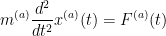
Our starting point is Newton’s second law  , which (partially) describes the motion of a particle
  of some fixed mass
  moving in the spatial domain . (Here we assume that the mass
  of a particle does not vary with time; in particular, our discussion will be purely non-relativistic in nature, though it is possible to derive a relativistic version of the Euler equations by variants of the arguments given here.) We write Newton’s second law as the ordinary differential equation

where  is the trajectory of the particle (thus
  denotes the position of the particle at time ), and
  is the force applied to that particle. If we write
  for the coordinates of the vector-valued function , and similarly write
  for the components of
  , we therefore have

where we adopt in this section the convention that the indices  are always understood to range from
  to .
to .
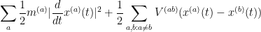
If one has some collection  particles instead of a single particle, indexed by some set of labels
  (e.g. the numbers from to
  , if there are a finite number of particles; for unbounded domains such as one can also imagine situations in which is infinite), then for each
  , the
, the  particle
  has some mass
  , some trajectory
  (with components
  ), and some force applied
  (with components
  , we thus have the equation of motion
or in components

In this section we adopt the convention that the indices  are always understood to range over the set of labels for the particles; in particular, their role should not be confused with those of the coordinate indices
  .
.
Newton’s second law does not, by itself, completely specify the evolution of a system of particles, because it does not specify exactly how the forces  depend on the current state of the system. For particles, the current state at a given time is given by the positions
  of all the particles
  , as well as their velocities
  ; we assume for simplicity that the particles have no further physical characteristics or internal structure of relevance that would require more state variables than these. (No higher derivatives need to be specified beyond the first, thanks to Newton’s second law. On the other hand, specifying position alone is insufficient to describe the state of the system; this was noticed as far back as Zeno in his paradox of the arrow, which in retrospect can be viewed as a precursor to Newton’s second law insofar as it demonstrated that the laws of motion needed to be second-order in time (in contrast, for instance, to Aristotlean physics, which was morally first-order in nature).) At a fundamental level, the dependency of forces on the current state are governed by the laws of physics for such forces; for instance, if the particles interact primarily through electrostatic forces, then one needs the laws of electrostatics to describe these forces. (In some cases, such as electromagnetic interactions, one cannot accurately model the situation purely in terms of interacting particles, and the equations of motion will then involve some additional mediating fields such as the electromagnetic field; but we will ignore this possibility in the current discussion for sake of simplicity.)
Fortunately, thanks to other laws of physics, and in particular Newton’s other two laws of motion, one can still obtain partial information about the forces without having to analyse the fundamental laws producing these forces. For instance, Newton’s first law of motion (when combined with the second) tells us that a single particle does not exert any force on itself; the net force on only arises from interaction with other particles ,  (for this discussion we neglect external forces, such as gravity, although one could easily incorporate such forces into this discussion; see Exercise 3 below). We will assume that the only forces present are pair interactions coming from individual pairs of particles
  ; it is theoretically possible that one could have more complicated interactions between, say, a triplet
  of particles that do not simply arise from the interactions between the three pairs ,
  ,
,  , but we will not consider this possibility here. We also assume that the net force on a particle is just the sum of all the interacting forces (i.e., the force addition law contains no nonlinear terms). This gives us a decomposition

of the net force on a particle into the interaction force  exerted on by another particle . Thus the equation of motion is now

Of course, this description is still incomplete, because we have not specified exactly what the interaction forces  are. But one important constraint on these forces is provided by Newton’s third law

This already gives some restrictions on the possible dynamics. For instance, it implies (formally, at least) that the total momentum

(which takes values in ) is conserved in time:


We will also assume that the interaction force between a pair  of particles is parallel to the displacement
  between the pair; in other words, we assume the torque
 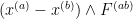 created by this force vanishes, thus

Here  is the exterior product on (which in three dimensions can be transformed if one wishes to the cross product, but is well defined in all dimensions). Algebraically,
  is the universal alternating bilinear form on ; in terms of the standard basis
  of , the wedge product
  of two vectors
  ,
,  is given by

and the vector space  is the formal span of the basic wedge products
  for
for  .
.
One consequence of the absence (4) of torque is the conservation of total angular momentum

(around the spatial origin  ). Indeed, we may calculate


Note that there is nothing special about the spatial origin ; the angular momentum

around any other point  is also conserved in time, as is clear from repeating the above calculation, or by combining the existing conservation laws for (3) and (5).
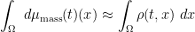
Now we pass from particle mechanics to continuum mechanics, by considering the limiting (bulk) behaviour of many particle systems as the number of particles per unit volume goes to infinity. (In physically realistic scenarios, will be comparable to Avagadro’s constant, which seems large enough that such limits should be a good approximation to the truth.) To make such limits, we assume that the distribution of particles (and various properties of these particles, such as their velocities and net interaction forces) are approximated in a certain bulk sense by continuous fields. For instance, the mass distribution of a system of particles at a given time is given by the discrete measure
where  denotes the Dirac measure (or distribution). We will assume that at each time , we have a “bulk” approximation

by some continuous measure  , where the density function
  is some smooth function of time and space, and
  denotes Lebesgue measure on . What does bulk approximation mean? One could work with various notions of approximation, but we will adopt the viewpoint of the theory of distributions (as reviewed for instance in these old lecture notes of mine) and consider approximation against test functions in spacetime, thus we assume that

for all spacetime test functions  . (One could also work with purely spatial test functions at each fixed time , or work with “infinitesimal” paralleopipeds or similar domains instead of using test functions; the arguments look slightly different when doing so, but the final equations of motion obtained are the same in all cases. See Exercise 1 for an example of this.) We will be deliberately vague as to what
  means, other than to say that the approximation should only be considered accurate (in the sense that it becomes exact in the limit
  ) when the test function
  exists at “macroscopic” (or “bulk”) spatial scales, in particular it should not oscillate with a wavelength that goes to zero as goes to infinity. (For instance, one certainly expects the approximation (7) to break down if one tries to test it on scales comparable to the mean spacing between particles.)
Applying (6) and evaluating the delta integrations, the approximation (8) becomes

In a physical liquid, particles in a given small region of space tend to move at nearly identical velocities (as opposed to gases, where Brownian motion effects lead one to expect velocities to be distributed stochastically, for instance in a Maxwellian distribution). To model this, we assume that there exists a smooth velocity field  for which we have the approximation
for all particles and all times . (When stochastic effects are significant, the continuum limit of the fluid will be the Boltzmann equations rather than the Euler or Navier-Stokes equations; however the latter equations can still emerge as an approximation of the former in various regimes. See also Remark 7 below.)
Implicit in our model of many-particle interactions is the conservation of mass: each particle has a fixed mass  , and no particle is created or destroyed by the evolution. This conservation of mass, when combined with the approximations (9) and (10), gives rise to a certain differential equation relating the density function
  and the velocity field
  . To see this, first observe from the fundamental theorem of calculus in time that

or equivalently (after applying (6) and evaluating the delta integrations)

for any test function (note that we make compactly supported in both space and time). By the chain rule and (10), we have

for any particle and any time , where  denotes the partial derivative with respect to the time variable,
  denotes the spatial gradient (with
  denoting partial differentiation in the
  coordinate), and
  denotes the Euclidean inner product. (One could also use notation here that avoids explicit use of Euclidean structure, for instance writing
  in place of
  , but it is traditional to use Euclidean notation in fluid mechanics.) This particular combination of derivatives
  appears so often in the subject that we will give it a special name, the material derivative
  :
:

We have thus obtained the approximation
which on insertion back into (12) yields

The material derivative  of a test function will still be a test function . Therefore we can use our field approximation (9) to conclude that

for all test functions . The left-hand side consists entirely of the limiting fields, so on taking limits we should therefore have the exact equation

We can integrate by parts to obtain

where  is the adjoint material derivative

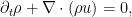
Since the test function was arbitrary, we conclude the continuity equation

or equivalently (and more customarily)

We will eventually specialise to the case of incompressible fluids in which the density is a non-zero constant in both space and time. (In some texts, one uses incompressibility to refer only to constancy of along trajectories:  . But in this course we always use incompressibility to refer to homogeneous incompressibility, in which is constant in both space and time.) In this incompressible case, the continuity equation (15) simplifies to a divergence-free condition on the velocity:
For now, though, we allow for the possibility of compressibility by allowing to vary in space and time. We also note that by integrating (15) in space, we formally obtain conservation of the total mass

since on differentiating under the integral sign and then integrating by parts we formally have
Of course, this conservation law degenerates in the incompressible case, since the total mass  is manifestly an infinite constant. (In periodic settings, for instance if one is working in instead of , the total mass
  is manifestly a finite constant in the incompressible case.)
Exercise 1
- (i) Assume that the spacetime bulk approximation (8) is replaced by the spatial bulk approximation

for any time and any spatial test function  . Give an alternate heuristic derivation of the continuity equation (15) in this case, without using any integration in time. (Feel free to differentiate under the integral sign.)
- (ii) Assume that the spacetime bulk approximation (8) is replaced by the spatial bulk approximation
for any time and any “reasonable” set  (e.g., a rectangular box). Give an alternate heuristic derivation of the continuity equation (15) in this case. (Feel free to introduce infinitesimals and argue non-rigorously with them.)
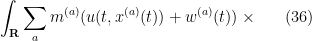
We can repeat the above analysis with the mass distribution (6) replaced by the momentum distribution

thus we now wish to exploit the conservation of momentum rather than conservation of mass. The measure  is a vector-valued measure, or equivalently a vector
  of scalar measures
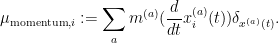
Instead of starting with the identity (11), we begin with the momentum counterpart

which on applying (17) and evaluating the delta integrations becomes

Using the product rule and (13), the left-hand side is approximately

Applying (1) and (10), we conclude

We can evaluate the second term using (9) to obtain

What about the first term? We can use symmetry and Newton’s third law (2) to write


Now we make the further physical assumption that the only significant interactions between particles are short-range interactions, in which  and
and  are very close to each other. With this hypothesis, it is then plausible to make the Taylor approximation

We thus have
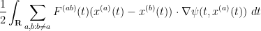
We write this in coordinates as

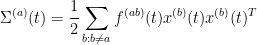
for  , where we use the Einstein convention that indices are implicitly summed over
  if they are repeated in an expression, and the stress
  on the particle at time is the rank
  -tensor defined by the formula

where  denote the components of . Recall from the torque-free hypothesis (4) that is parallel to
  , thus we could write
  for some scalar
  . Thus we have

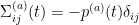
In particular, we see that the torque-free hypothesis makes the stress tensor symmetric:

To proceed further, we make the assumption (similar to (9)) that the stress tensor  (or more precisely, the measure
  ) is approximated in the bulk by a smooth tensor field
  (with components
  for
for  ), in the sense that

The tensor  is known as the Cauchy stress tensor. Since is symmetric in
  , the right-hand side of (21) is also symmetric in , which by the arbitrariness of implies that the tensor
  is symmetric also:

This is also known as Cauchy’s second law of motion.
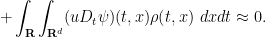
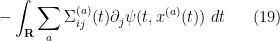
Inserting (19) into (21), we arrive at

for any test function and . Taking limits as we obtain the exact equation

and then integrating by parts we have
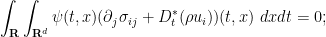
as the test function is arbitrary, we conclude the Cauchy momentum equation

From the Leibniz rule (in an adjoint form) we see that

using (14) we can thus also write the Cauchy momentum equation in the more conventional form
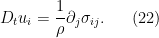
(This is a dynamical version of Cauchy’s first law of motion.)
To summarise so far, the unknown density field and velocity field obey two equations of motion: the continuity equation (15) (or (14)) and the momentum equation (22). As the former is a scalar equation and the latter is a vector equation, this is  equations for unknowns, which looks good – so long as the stress tensor is known. However, the stress tensor is not given to us in advance, and so further physical assumptions on the underlying fluid are needed to derive additional equations to yield a more complete set of equations of motion.
One of the simplest such assumptions is isotropy – that, in the vicinity of a given particle at a given point in time, the distribution of the nearby particles (and of the forces  ) is effectively rotationally symmetric, in the sense that rotation of the fluid around that particle does not significantly affect the net stresses acting on the particle. To give more mathematical meaning to this assumption, let us fix
  and , and let us set to be the spatial origin
  for simplicity. In particular the stress tensor
  now simplifies a little to

viewing this tensor as a  symmetric matrix, we can also write
where we now think of the vector as a -dimensional column vector, and  denotes the transpose of
  .
.
Imagine that we rotate the fluid around this spatial origin using some rotation matrix  , thus replacing with
  (and hence
  is replaced with
  ). If we assume that interaction forces are rotationally symmetric, the interaction scalars
  should not be affected by this rotation. As such, would be replaced with
  . If we assume isotropy, though, this rotated fluid should generate the same stress as the original fluid, thus we have

for all rotation matrices  , that is to say that commutes with all rotations. This implies that all eigenspaces of are rotation-invariant, but the only rotation-invariant subspaces of are
  and . Thus the spectral decomposition of the symmetric matrix only involves a single eigenspace , or equivalently is a multiple of the identity. In coordinates, we have
for some scalar  (known as the pressure exerted on the particle ), where
  denotes the Kronecker delta (the negative sign here is for compatibility with other physical definitions of pressure). Passing from the individual stresses to the stress field , we see that is also rotationally invariant and thus is also a multiple of the identity, thus

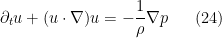
for some field 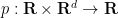 , which we call the pressure field, and which we assume to be smooth. The equations (15), (22) now become the Euler equations

This is still an underdetermined system, being equations for  unknowns (two scalar fields
  and one vector field ). But if we assume incompressibility (normalising
  for simplicity), we obtain the incompressible Euler equations


Without incompressibility, one can still reach a determined system of equations if one postulates a relationship (known as an equation of state) between the pressure  and the density (in some physical situations one also needs to introduce further thermodynamic variables, such as temperature or entropy, which also influence this relationship and obey their own equation of motion). Alternatively, one can proceed using an analysis of the energy conservation law, similar to how (15) arose from conservation of mass and (22) arose from conservation of momentum, though at the end of the day one would still need an equation of state connecting energy density to other thermodynamic variables. For details, see Exercise 4 below.
Now we consider relaxing the assumption of isotropy in the stress. Many fluids, in addition to experiencing isotropic stress coming from a scalar pressure field, also experience additional shear stress associated to strain in the fluid – distortion in the shape of the fluid arising from fluctuations in the velocity field. One can thus postulate a generalisation to (23) of the form

where  is some function of the velocity
  at the point
  in spacetime, as well as the first derivatives
  , that arises from changes in shape. (Here, we assume here that the response to stress is autonomous – it does not depend directly on time, location, or other statistics of the fluid, such as pressure, except insofar as those variables are related to the quantities
  and
and  . One can of course consider more complex models in which there is a dependence on such quantities or on higher derivatives
  , etc. of the velocity, but we will not do so here.)
It is a general principle in physics that functional relationships between physical quantities, such as the one in (27), can be very heavily constrained by requiring the relationship to be invariant with respect to various physically natural symmetries. This is certainly the case for (27). First of all, we can impose Galilean invariance: if one changes to a different inertial frame of reference, thus adding a constant vector  to the velocity field (and not affecting the gradient
  at all), this should not actually introduce any new stresses on the fluid. This leads to the postulate

for any , and hence  should not actually depend on the velocity and should only depend on the first derivative. Thus we now write
  for
for 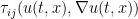 (thus is now a function from
  to ).
to ).
If  then there should be no additional shear stress, so we should have
  . We now make a key assumption that the fluid is a Newtonian fluid, in that the linear term in the Taylor expansion of
  dominates, or in other words we assume that is a linear function of . (One can certainly study the mechanics of non-Newtonian fluids as well, in which depends nonlinearly on , or even on past values of , but these are no longer governed by the Navier-Stokes equations and will not be considered further here.) One can also think of as a linear map from the space of
  matrices (which is the space where takes values) to the space of matrices. In coefficients, this means we are postulating a relationship of the form
for some constants  (recall we are using the Einstein summation conventions). This looks like a lot of unspecified constants, but again we can use physical principles to impose significant constraints. Firstly, because stress is symmetric in
  and
and  , the coefficients must also be symmetric in and :
  . Next, let us for simplicity set to be the spatial origin , and consider a rotating velocity field of the form

for some constant-coefficient anti-symmetric matrix , or in coordinates
The derivative field  is then just the anti-symmetric
  . This corresponds to fluids moving according to the rotating trajectories
  , where
  denotes the matrix exponential. (For instance, in two dimensions, the velocity field
  gives rise to trajectories
  ,
,  corresponding to counter-clockwise rotation around the origin.)
Exercise 2 When is anti-symmetric, show that the matrix  is orthogonal for all , thus

for all  , where denotes the identity matrix. (Hint: differentiate the expressions appearing in the above equation with respect to time.) Also show that
  is a rotation matrix, that is to say an orthogonal matrix of determinant
  .
.
As is orthogonal, it describes a rigid motion. Thus this rotating motion does not change the shape of the fluid, and so should not give rise to any shear stress. That is to say, the linear map should vanish when applied to an anti-symmetric matrix, or in coordinates  . Another way of saying this is that
  only depends on through its symmetric component
  , known as the rate-of-strain tensor (or the deformation tensor). (The anti-symmetric part
  does not cause any strain, but instead measures the infinitesimal rotation the fluid; up to trivial factors such as
  , it is essentially the vorticity of the fluid, which will be an important field to study in subsequent notes.)
To constrain the behaviour of further, we introduce a hypothesis of rotational (and reflectional) symmetry. If one rotates the fluid by a rotation matrix around the origin, then if the original fluid had a velocity of at , the new fluid should have a velocity of  at
at  , thus the new velocity field
  is given by the formula
and the derivative  of this velocity field at the origin is then related to the original derivative by the formula

Meanwhile, as discussed in the analysis of the isotropic case, the new stress  at the origin is related to the original stress by the same relation:

This means that the linear map is rotationally equivariant in the sense that

for any matrix . Actually the same argument also applies for reflections, so one could also take in the orthogonal group  rather than the special orthogonal group.
This severely constrains the possible behaviour of . First consider applying to the rank matrix  , where
  is the first basis (column) vector of . The equivariant property (28) then implies that
  is invariant with respect to any rotation or reflection of the remaining coordinates
  . As in the isotropic analysis, this implies that the lower right
  minor of is a multiple of the identity; when
  it also implies that the upper right entries
  or lower left entries
  for
for  also vanish (one can also obtain this by applying (28) with the reflection in the
  variable). Thus we have
for some constant scalars  (known as the dynamic viscosity and second viscosity respectively); in matrix form we have
where  is the identity matrix. Applying equivariance, we conclude that

for any unit vector  ; applying the spectral theorem this implies that
for any symmetric matrix . Since  is already known to vanish for non-symmetric matrices, upon decomposing a general matrix into the symmetric part
  and anti-symmetric part
  (with the latter having trace zero) we conclude that

for an arbitrary matrix . In particular

In the incompressible case  , the second term vanishes, and this equation simply says that the shear stress is proportional to the (rate of) strain.
Inserting the above law back into (27) and then (15), (22), we obtain the Navier-Stokes equations

where  is the spatial Laplacian. In the incompressible case, setting
  (this ratio is known as the kinematic viscosity), and also normalising for simplicity, this simplifies to the incompressible Navier-Stokes equations

Of course, the incompressible Euler equations arise as the special case when the viscosity  is set to zero. For physical fluids, is positive, though it can be so small that the Euler equations serve as a good approximation. Negative values of
  are mathematically possible, but physically unrealistic for several reasons (for instance, the total energy of the fluid would increase over time, rather than dissipate over time) and also the equations become mathematically quite ill-behaved in this case (as they carry essentially all of the pathologies of the backwards heat equation).
Exercise 3 In a constant gravity field oriented in the direction  , each particle will experience an external gravitational force
  , where
  is a fixed constant. Argue that the incompressible Euler equations in the presence of such a gravitational field should be modified to

and the incompressible Navier-Stokes equations should similarly be modified to

Exercise 4
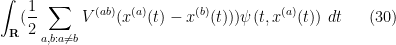
- (i) Suppose that in an -particle system, the force
 between two particles is given by the conservative law

for some smooth potential function  , which we assume to obey the symmetry
  to be consistent with Newton’s third law. Show that the total energy
is conserved in time (that is to say, the time derivative of this quantity vanishes). Here of course we use  to denote the Euclidean magnitude of a vector .
- (ii) Assume furthermore that in the large limit, we have the velocity approximation (10), the stress approximation (21), and the isotropy condition (23). Assume all interactions are short-range. Assume we also have a potential energy approximation
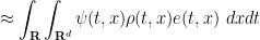
for all test functions and some smooth function  (usually called the specific internal energy). By analysing the energy distribution

in analogy with the previous analysis of the mass distribution  and momentum distribution
  , make a heuristic derivation of the energy conservation law

or equivalently

where the energy density  is defined by the formula

(that is to say, is the sum of the kinetic energy density  and the internal energy density
  ). Conclude in particular that the total energy

is formally conserved in time.
- (iii) In addition to the previous assumptions, assume that there is a functional relationship between the specific energy density
 and the density
  , in the sense that there is a smooth function
  such that

at all points in spacetime and all physically relevant configurations of particles. (In particular, we are in the compressible situation in which we allow the density to vary.) By dilating the position variables  by a scaling factor
  , scaling the test function appropriately, and working out (via (9)) what the scaling does to the density function , generalise (30) to


Formally differentiate this approximation with respect to  at
at  and use (29), (20), (21), (23) to heuristically derive the equation of state

- (iv) Give an alternate derivation of the energy conservation law (31) from the equations (24), (25), (33), (34). (Note that as the fluid here is compressible, one cannot use any equations in this post that rely on an incompressibility hypothesis.)
- (v) Suppose the functional relationship (33) uses a function of the form

for some constant  (the specific energy density at equilibrium) and some large and positive ; physically, this represents a fluid which is nearly incompressible in the sense that it is very resistant to having its density deviate from . Assuming that the pressure stays bounded and is large, heuristically derive the approximations

and

Formally, in the limit  , we thus heuristically recover an incompressible fluid with a constant specific energy density
  . In particular the contributions of the specific energy to the energy conservation law (31) may be ignored in the incompressible case thanks to (24).
Remark 5 In the literature, the relationship between the functional relationship (33) and the equation of state (34) is usually derived instead using the laws of thermodynamics. However, as the above exercise demonstrates, it is also possible to recover this relationship from first principles. In the case of an (isoentropic) ideal gas, the laws of thermodynamics can be used to establish an equation of state of the form  for some constants
  with
with  , as well as the corresponding functional relationship
  , so that the internal energy density is
  . This is of course consistent with (33) and (34), after choosing appropriately.
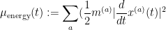
Exercise 6 Suppose one has a (compressible or incompressible) fluid obeying the velocity approximation (10), the stress approximation (21), the isotropy condition (23), and the torque free condition (4). Assume also that all interactions are short range. Derive the angular momentum equation
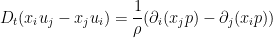
for  in two different ways:
(c) Conclude in particular that the total angular momentum
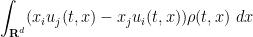
is formally conserved in time.
Remark 7 In this set of notes we made the rather strong assumption (10) that the velocities of particles could be approximated by a smooth function of their time and position. In practice, most fluids will violate this hypothesis due to thermal fluctuations in the velocity. However, one can still proceed with a similar derivation assuming that the velocities behave on the average like a smooth function , in the sense that


for any test function . The approximation (13) now has to be replaced by the more general

where

is the deviation of the particle velocity from its mean. The second term in (18) now needs to be replaced by the more complicated expression

From (35), (9) one has

for any test function . This allows us to heuristically drop the cross terms from (36) involving a single factor of  , and simplify this expression (up to negligible errors) as


Repeating the analysis after (18), one eventually arrives again at (19), except that one has to add an additional term
to the stress tensor of a single particle . However, this term is still symmetric, and one can still continue most of the heuristic analysis in this post after suitable adjustments to the various physical hypotheses (for instance, assuming some form of the molecular chaos hypothesis to be able to neglect some correlation terms between and other quantities). We leave the details to the interested reader.


41 comments
Comments feed for this article
3 September, 2018 at 5:10 pm
Anonymous
Is the argument between (19) and (20) entirely mathematical apart from leaning on isotropy as a physical assumption?
3 September, 2018 at 6:15 pm
Terence Tao
(I presume you now mean the argument between (20) and (21); the equation numbering changed recently due to some further edits.)
In addition to isotropy, a number of other physical assumptions were also used, including: assuming short-range, torque-free pair interactions are the only forces present, and also that the interaction strengths are rotation-invariant (they do not depend on the orientation of
  ). They also require various error terms in the approximations
  appearing in the text to be negligible in various specific senses. It may be though that one could derive the Cauchy momentum equation with fewer physical assumptions than the ones used here; I was not aiming for minimality of assumption in these notes.
4 September, 2018 at 5:19 am
Anonymous
Actually that specific argument is now between (21) and (22). I believe it’s only isotropy; I’d appreciate being corrected since multiple physics-oriented texts are vague on whether d=3 is a required assumption for that argument.
3 September, 2018 at 5:28 pm
Biruk Alemayehu petros
What will be the implication if there is periodic smooth unique solution for NSE? The solution has decaying amplitude in time and viscosity, periodic in space with oscillating term moving with phase velocity of decaying in time and viscosity. Partial result is being published. But the solution published is not unique. Unpublished solution is unique smooth. Am an electrical engineer and need help. Am sure you are busy and not interested in this kind of request. But remember hardy and ramanujan when reading this comment.
I respect your job for public understanding of important topics
Biruk Alemayehu Petros
5 September, 2018 at 11:28 am
Biruk Alemayehu petros
Smooth unique periodic solution for Navier Stokes equations. The solution suggests the turbulent term and laminar term move with the same velocity. Meaning if move along the fluids overall flow you can see the vortex being stationary and decaying in time and finally vanishes due to viscosity.
http://vixra.org/abs/1809.0088
5 September, 2018 at 11:33 am
Biruk Alemayehu petros
http://vixra.org/abs/1809.0088
Is unique smooth periodic solution defined in all times and spaces.
3 September, 2018 at 11:36 pm
Anonymous
Is it possible to assign a well-defined “asymptotic distribution” for zeros (for large zeros
  ), such that the dynamics of the zeros can give a corresponding evolution equation (or “flow”) for the asymptotic distribution “density” of the zeros ?
 zeros (considered now as a density of a “fluid”) ?
If so, is it possible to get a concrete form for the equations governing the dynamics of this “asymptotic density” of
4 September, 2018 at 6:13 am
Terence Tao
Continuum limits of the zeta function (and the zeroes thereof) at the “macroscopic” or “bulk” scale 1 are discussed in this previous blog post: https://terrytao.wordpress.com/2015/03/01/254a-supplement-7-normalised-limit-profiles-of-the-log-magnitude-of-the-riemann-zeta-function-optional/ . The heat flow is degenerate that this scale though: after any fixed positive time, the continuum limit “freezes” to a uniform distribution.
To retain an interesting dynamics, one should instead renormalise at the “microscopic” scale (the scale of the mean spacing between zeroes), in which case one does not obtain a continuum limit, but instead a stochastic limit which is conjecturally distributed according to the GUE hypothesis. The equations of heat flow are unaffected by this rescaling. The GUE distribution is not invariant under this heat flow (it is instead invariant under the
  analogue of this
  flow, namely Dyson Brownian motion); the evolution of this distribution is in principle explicit, but probably quite messy.
4 September, 2018 at 4:10 am
Lior Silberman
Concerning the hypothesis that the interparticle forces are aligned with the displacement vectors (just before equation (4)), this follows immediately if you assume isotropy of the laws of physics, since rotating the system in the hyperplane perpendicular to the displacement vector leaves the two pricked fixed and hence must fix the force between them.
4 September, 2018 at 6:18 am
Terence Tao
I guess it would follow more from the rotational invariance of the laws of physics combined with a hypothesis that the internal state of each particle is also isotropic (physically indistinguishable from any rotation of that particle, after applying a Galilean transform to normalise the position and velocity of the particle to vanish). If for instance each particle had a strong magnetic moment or spin then one could conceivably have non-trivial torque between two particles even if the laws of physics remain perfectly rotationally symmetric.
4 September, 2018 at 6:28 am
Lior Silberman
Yes — I’m assuming the particles themselves have no internal structure. But this assumption was effectively made when the force was stated to only depends on the locations of the particles.
[Fair enough – I’ll add a comment to that effect in the post. -T]
4 September, 2018 at 6:12 am
Anonymous
There is a typo in the sentence:
…”particles that do not simply arise from the interactions between the three pairs”. The P_b, should be P^(b).
[Corrected, thanks – T.]
4 September, 2018 at 12:41 pm
Anonymous
In the displayed formula (below (4)) defining the wedge product, the first summation should be also on .
.
[Corrected, thanks – T.]
4 September, 2018 at 1:34 pm
Darius
Absolute genius-level work. I’m pursuing physics, and have seen nothing like this.
4 September, 2018 at 4:10 pm
Anonymous
That’s because, presumably, you read material written by physicists, not mathematicians.
4 September, 2018 at 11:21 pm
Anonymous
It seems that this model can be refined by additional stochastic modeling of the fluid particles (i.e. molecules) for their rotations, vibrations and time-varying deformations (via inter-molecular interactions). Perhaps temperature distribution is the simplest scalar field describing such stochastic refinement (using the specific heat concept to describe the internal thermal energy contribution).
5 September, 2018 at 7:32 am
Terence Tao
Yes, this derivation certainly assumes far stronger conditions on the microscopic interactions than are actually needed to (heuristically) derive the Euler or Navier-Stokes equations, which are somewhat (though certainly not completely) universal in nature, in the sense that they seem to be a good approximation for a fairly wide class of fluids and physical regimes, including some that fail one or more of the assumptions given in this set of notes. I chose this particular derivation for pedagogical reasons, as I wanted to illustrate the point that it is in fact possible to derive these bulk fluid equations from the first principles of Newtonian mechanics, albeit with some rather restrictive hypotheses on the microscopic interactions. As you say, it is likely that some of these hypotheses can be relaxed while still being able to obtain a largely similar derivation.
In fluid mechanics textbooks one will find other derivations of these fluid laws that are not based so much on microscopic interactions but instead on bulk laws of physics, such as bulk conservation laws and the laws of thermodynamics. These derivations are significantly more robust than the ones given here, in that they will (heuristically, at least) apply to a much wider class of fluids and physical regimes. But they also require more physics prerequisites than I wished to give in this course, which (aside from this particular set of notes) will be focused purely on the mathematical side of things. In particular, I did not wish to digress into a discussion of the laws of thermodynamics.
5 September, 2018 at 7:36 am
Martin
There is progress on the Millennium problem by Buckmaster, Colombo and Vicol:
https://arxiv.org/abs/1809.00600
6 September, 2018 at 9:15 pm
roland5999
Having derived a big deal of entertainment (and instruction) from the above,
humble me wonders (tongue in cheek) how pedagogically advisable it is to hand out the dessert before the main dish?
After all, the physics side of things (the pudding) could be looking more desirable (to some)
as opposed to the difficult math side (the meat).
“if you don’t eat your meat, you can’t have any pudding!”
:) r.
8 September, 2018 at 1:27 pm
Anonymous
This is not a physical derivation of Navier Stokes but a mathematical one. For the physical derivation one needs to solve the Boltzmann equation.
8 September, 2018 at 4:43 pm
Terence Tao
When the effects of stochastic fluctuations in velocity are significant then one indeed has to pass through the Boltzmann equations first before deriving hydrodynamic equations such as Euler and Navier-Stokes. But here I am assuming that such effects are negligible (see equation (10)) which allows one to take a shortcut and jump from Newtonian mechanics directly to the fluid equations without involving the Boltzmann equations. Admittedly this is a rather restrictive assumption that reduces the number of physical fluids and regimes to which the derivation in this post is valid, but I find it to be simpler pedagogically than the full-blown derivation (in particular avoiding the need to introduce laws of thermodynamics), and still is a legitimate derivation of these fluid equations from more fundamental laws of physics in these more restricted regimes. I’ve added a comment in the post as to how the Boltzmann equations will need to be deployed in the presence of stochastic velocity fluctuations, though.
9 September, 2018 at 6:22 am
Anonymous
You mean collisions????
Or does your derivation simply ignores molecular chaos???
9 September, 2018 at 7:12 am
Terence Tao
The interaction forces in the model in the post can effectively generate collisions, though the hypotheses of the model are that these collisions do not cause significant deviation in velocity from the mean velocity
  . If one takes these additional deviations into account then one would obtain a further contribution to the stress tensor, but will ultimately arrive at the same hydrodynamic limits (with the pressure
  containing an additional term arising from those deviations), if one makes appropriate assumptions on the homogeneity, chaos, and magnitude of these deviations.
Basically, the pedagogy in this post was to find a set of physical hypotheses that would allow one to arrive at hydrodynamic equations from Newtonian first principles as rapidly as possible, without need for additional prerequisite material from other laws of physics (such as thermodynamics) or from probability. As I mentioned previously, these hypotheses are quite restrictive; however, as pointed out by other commenters, the derivation can be adapted to handle wider classes of fluids, including those with significant stochastic velocity fluctuation, at the cost of complicating the analysis somewhat, for instance by having to first derive the Boltzmann equations as an intermediate approximation. (Also, I find it an instructive point that while such velocity fluctuations is a notable feature of real-world fluids, they is not strictly necessary as an ingredient for the derivation of hydrodynamic equations.)
9 September, 2018 at 7:32 am
Anonymous
How about a simple Molecular Dynamics Simulation? Since you’re derivation seems to resemble an MD simulation (pair interaction etc..)
9 September, 2018 at 7:40 am
Anonymous
Also how do you evaluate transport coefficients?? For instance the coefficient of viscosity?
10 September, 2018 at 4:08 am
Anonymous
I agree, without a closed equation for the corresponding transport coefficient this derivation is insufficient.
10 September, 2018 at 8:14 am
Terence Tao
The existence of transport coefficients here arise from the hypothesis that the fluid is Newtonian; they are not calculated or derived from the other physical quantities in the model, though as discussed in the post the Galilean and rotational symmetry hypotheses do significantly constrain how these coefficients depend on the indices
  , in that these coefficients are completely determined by the two viscosity parameters
  . However, these axioms are not enough by themselves to calculate these latter parameters exactly. It is true though that the derivation of Navier-Stokes from Boltzmann would, in principle at least, allow one to evaluate these parameters in terms of other parameters of the Boltzmann model, which in turn could in principle be derived from Newtonian primitives such as the form of the pair interaction forces
  . However, the philosophy adopted in this post is to take the hypothesis of a Newtonian fluid as a primitive axiom, rather than as a property to be derived from more fundamental laws of physics, in order to arrive at the hydrodynamic equations as quickly as possible. [This is similar to how Hooke’s law is used to derive the equations of linear elasticity.]
Basically, while I would indeed like the derivation of the fluid equations to be 100% from Newtonian first principles, this was a secondary pedagogical consideration compared with the primary objective of keeping the derivation short and requiring minimal physics prerequisites. The assumption of bulk laws of physics such as that of a Newtonian fluid was thus a compromise to further the primary aim at the expense of the secondary one.
p.s. I have now added a final remark (Remark 7) to the post regarding the addition of velocity fluctuations to the model.
4 December, 2020 at 7:49 am
amiteshs4
Only to add on to an excellent answer, but I think this could be mentioned. From the Boltzmann equations, one obtains the Navier-Stokes equation only as a first order approximation (typically by a Chapman-Enskog expansion). Higher-order equations such as the Burnett equations do exist (of which the Navier-Stokes equations are a subset). And one could create hierarchically more complicated descriptions using the Boltzmann equations, as well as using the BBGKY hierarchy from the Liouville equations. In engineering, statistical mechanical descriptions that add on to (or even replace continuum level descriptions), are becoming more common especially in applications concerning rarefied gas dynamics and nanofluid transport.
26 December, 2020 at 6:53 am
Anonymous
Also the Chapman-Enskog method delivers a conservation law for kinetic energy which is not present in Mr Tao’s derivation.
24 September, 2018 at 1:28 am
august
Note from a physicist: the two dimensional case is usually considered pathological. The expressions used (Kubo formula) to calculate the viscosity diverge in two dimensions. I suspect that our author knows this, but for mathematicians reading along it shows that the formal machine is very fragile. The breakdowns are logarithmic, but show that the idea of local hydrodynamics without memory is not valid in 2d geometries.
24 September, 2018 at 2:00 am
Gabe
That’s used in molecular dynamics, yes? But there is a lot of math and engineering work done using the two-dimensional case.
2 October, 2018 at 3:47 pm
254A, Notes 2: Weak solutions of the Navier-Stokes equations | What's new
[…] any smooth function (cf. the material derivative used in Notes 0). Thus, one can rewrite the initial value problem (9) […]
6 November, 2018 at 3:32 am
biruk
Trust me there is counter example for mellinium prize problem. Available at researchgate. I propose we need to modify navier stokes equations to be valid discription of natural phenomenon.
https://www.researchgate.net/publication/328249810_Non-Unique_Smooth_Periodic_Solutions_in_the_absence_of_external_Force_for_Navier_Stokes_Three_Dimensional_Equation_defined_on_a_Torus
18 November, 2018 at 3:51 am
Anonymous
I think that there should not be a \partial_j in the formula just before (22).
[Corrected, thanks – T].
28 November, 2018 at 1:58 pm
254A, Notes 3: Local well-posedness for the Euler equations | What's new
[…] any smooth function (cf. the material derivative used in Notes 0). Thus, one can rewrite the initial value problem (9) […]
16 December, 2018 at 2:37 pm
255B, Notes 1: The Lagrangian formulation of the Euler equations | What's new
[…] Eulerian coordinates. However, if one reviews the physical derivation of the Euler equations from 254A Notes 0, before one takes the continuum limit, the fundamental unknowns were not the velocity field or the […]
3 January, 2019 at 2:11 am
titus
Are there any reference (maybe some of your lecture notes ?) on how to manipulate adjoint differential operators and the Leibniz rule ?
3 January, 2019 at 10:16 am
Terence Tao
The adjoint Leibniz rule, as the name suggests, is simply the adjoint of the usual Leibniz rule. For instance, starting with the usual Leibniz rule
for arbitrary test functions , if one integrates against another test function
  to get
and then integrates by parts again to move derivatives off of , thus
one recovers the adjoint Leibniz rule since
since  was arbitrary.
To put it another way: if is the operation of multiplying
  by
by  , the usual Leibniz rule reads
  , which on taking adjoints (or transposes) gives
  , which when unpacked and rearranged is the adjoint Leibniz rule.
30 July, 2020 at 4:35 am
Dmitri Gorskine
Dear professor Terence Tao, I found exact analytical general solution non steady 3D Navier-Stokes equation for incompressible flow. It was amazing, but solution for Navier-Stokes equation coefficient viscosity equal zero is not solution for 3D Euler equation. I don’t understand why?
27 May, 2022 at 7:36 am
Diego.Y.
I solved problem 1 by taking time derivative on both sides of approximation and pass derivative under integration. But doing in this way feels like I am not using mass conservation as my starting point. Similarly, I can use the same technique to obtain (22) from a space approximation version of (21) (of course requiring smoothness in space-time) and, as in the case of mass, I am not using the momentum conservation. I am not sure if this is correct or there is something I am missing. Any help would be appreciated.
[If you used the fact that the particle masses are constants (not depending on time), then you have used mass conservation. Similarly, if you have used Newton’s third law, then you have used momentum conservation – T.]
27 May, 2022 at 12:38 pm
Anonymous
Instead of the traditional interpretation of Newton’s second law as an equation for the computation of the momentum from a given force, it is possible to interpret this law as a definition(!) of the concept of “applied force” as the time rate of the concept of “momentum” (thus making Newton’s second law interpreted as “Newton’s definition of force” from the momentum).