
You are currently browsing the tag archive for the ‘twin primes’ tag.
Just a brief post to record some notable papers in my fields of interest that appeared on the arXiv recently.
- “A sharp square function estimate for the cone in
“, by Larry Guth, Hong Wang, and Ruixiang Zhang. This paper establishes an optimal (up to epsilon losses) square function estimate for the three-dimensional light cone that was essentially conjectured by Mockenhaupt, Seeger, and Sogge, which has a number of other consequences including Sogge’s local smoothing conjecture for the wave equation in two spatial dimensions, which in turn implies the (already known) Bochner-Riesz, restriction, and Kakeya conjectures in two dimensions. Interestingly, modern techniques such as polynomial partitioning and decoupling estimates are not used in this argument; instead, the authors mostly rely on an induction on scales argument and Kakeya type estimates. Many previous authors (including myself) were able to get weaker estimates of this type by an induction on scales method, but there were always significant inefficiencies in doing so; in particular knowing the sharp square function estimate at smaller scales did not imply the sharp square function estimate at the given larger scale. The authors here get around this issue by finding an even stronger estimate that implies the square function estimate, but behaves significantly better with respect to induction on scales.
- “On the Chowla and twin primes conjectures over
“, by Will Sawin and Mark Shusterman. This paper resolves a number of well known open conjectures in analytic number theory, such as the Chowla conjecture and the twin prime conjecture (in the strong form conjectured by Hardy and Littlewood), in the case of function fields where the field is a prime power
which is fixed (in contrast to a number of existing results in the “large
” limit) but has a large exponent
. The techniques here are orthogonal to those used in recent progress towards the Chowla conjecture over the integers (e.g., in this previous paper of mine); the starting point is an algebraic observation that in certain function fields, the Mobius function behaves like a quadratic Dirichlet character along certain arithmetic progressions. In principle, this reduces problems such as Chowla’s conjecture to problems about estimating sums of Dirichlet characters, for which more is known; but the task is still far from trivial.
- “Bounds for sets with no polynomial progressions“, by Sarah Peluse. This paper can be viewed as part of a larger project to obtain quantitative density Ramsey theorems of Szemeredi type. For instance, Gowers famously established a relatively good quantitative bound for Szemeredi’s theorem that all dense subsets of integers contain arbitrarily long arithmetic progressions
. The corresponding question for polynomial progressions
is considered more difficult for a number of reasons. One of them is that dilation invariance is lost; a dilation of an arithmetic progression is again an arithmetic progression, but a dilation of a polynomial progression will in general not be a polynomial progression with the same polynomials
. Another issue is that the ranges of the two parameters
are now at different scales. Peluse gets around these difficulties in the case when all the polynomials
, so that one can still run a density increment argument efficiently. To resolve the second difficulty one needs to find a quantitative concatenation theorem for Gowers uniformity norms. Many of these ideas were developed in previous papers of Peluse and Peluse-Prendiville in simpler settings.
- “On blow up for the energy super critical defocusing non linear Schrödinger equations“, by Frank Merle, Pierre Raphael, Igor Rodnianski, and Jeremie Szeftel. This paper (when combined with two companion papers) resolves a long-standing problem as to whether finite time blowup occurs for the defocusing supercritical nonlinear Schrödinger equation (at least in certain dimensions and nonlinearities). I had a previous paper establishing a result like this if one “cheated” by replacing the nonlinear Schrodinger equation by a system of such equations, but remarkably they are able to tackle the original equation itself without any such cheating. Given the very analogous situation with Navier-Stokes, where again one can create finite time blowup by “cheating” and modifying the equation, it does raise hope that finite time blowup for the incompressible Navier-Stokes and Euler equations can be established… In fact the connection may not just be at the level of analogy; a surprising key ingredient in the proofs here is the observation that a certain blowup ansatz for the nonlinear Schrodinger equation is governed by solutions to the (compressible) Euler equation, and finite time blowup examples for the latter can be used to construct finite time blowup examples for the former.
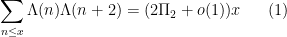
Kaisa Matomaki, Maksym Radziwill, and I have uploaded to the arXiv our paper “Correlations of the von Mangoldt and higher divisor functions I. Long shift ranges“, submitted to Proceedings of the London Mathematical Society. This paper is concerned with the estimation of correlations such as
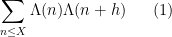
for medium-sized 


then this would easily imply the twin prime conjecture.
The (first) Hardy-Littlewood conjecture asserts an asymptotic
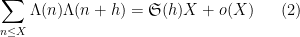
as 

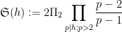
when 
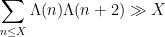
is (half of) the twin prime constant. See for instance this previous blog post for a a heuristic explanation of this conjecture. From the previous discussion we see that (2) for 

Needless to say, apart from the trivial case of odd 


The first results in this direction were by van der Corput and by Lavrik, who established such a result with 


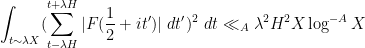
Our arguments initially proceed along standard lines. One can use the Hardy-Littlewood circle method to express the correlation in (2) as an integral involving exponential sums 


for any “minor arc” 


![{[x, x + x^{1/6+\varepsilon}]}](https://s0.wp.com/latex.php?latex=%7B%5Bx%2C+x+%2B+x%5E%7B1%2F6%2B%5Cvarepsilon%7D%5D%7D&bg=ffffff&fg=000000&s=0&c=20201002)
The next step (following some ideas we found in a paper of Zhan) is to rewrite this estimate not in terms of the exponential sums 
for any 

The next step, which is again standard, is the use of the Heath-Brown identity (as discussed for instance in this previous blog post) to split up 


![{[X^\varepsilon, X^{-\varepsilon} H]}](https://s0.wp.com/latex.php?latex=%7B%5BX%5E%5Cvarepsilon%2C+X%5E%7B-%5Cvarepsilon%7D+H%5D%7D&bg=ffffff&fg=000000&s=0&c=20201002)


for “typical” ordinates 

At this point, having exhausted all the Dirichlet polynomial estimates that are usefully available, we return to “physical space”. Using some further Fourier-analytic and oscillatory integral computations, we can estimate the left-hand side of (3) by an expression that is roughly of the shape
The phase 


In a sequel to this paper, we will use a somewhat different method to reduce 


The twin prime conjecture, still unsolved, asserts that there are infinitely many primes 

as 

Because
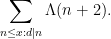
One can give a heuristic justification of the asymptotic (1) (and hence the twin prime conjecture) via sieve theoretic methods. Recall that the von Mangoldt function can be decomposed as a Dirichlet convolution

where 

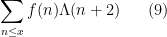
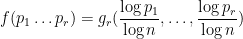
To compute this double sum, it is thus natural to consider sums such as
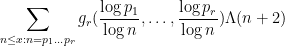
or (to simplify things by removing the logarithm)
The prime number theorem in arithmetic progressions suggests that one has an asymptotic of the form
where 


for
and so we heuristically have

The Dirichlet series

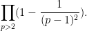
has an Euler product factorisation
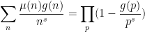
for 
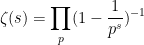
for the Riemann zeta function, and recalling that 

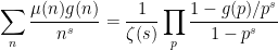
has a simple zero at

From this and standard multiplicative number theory manipulations, one can calculate the asymptotic
which concludes the heuristic justification of (1).
What prevents us from making the above heuristic argument rigorous, and thus proving (1) and the twin prime conjecture? Note that the variable 


However, because of the averaging effect of the summation in 


for various sieve weights 

which is off from (1) by a factor of about 
It has been difficult to improve upon the Bombieri-Vinogradov theorem in its full generality, although there are various improvements to certain restricted versions of the Bombieri-Vinogradov theorem, for instance in the famous work of Zhang on bounded gaps between primes. Nevertheless, it is believed that the Elliott-Halberstam conjecture (EH) holds, which roughly speaking would mean that (3) now holds for almost all 


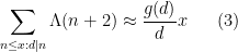
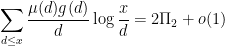
In two papers from the 1970s (which can be found online here and here respectively, the latter starting on page 255 of the pdf), Bombieri developed what is now known as the Bombieri asymptotic sieve to clarify the situation more precisely. First, he showed that on the Elliott-Halberstam conjecture, while one still could not establish the asymptotic (1), one could prove the generalised asymptotic

for all natural numbers 


These functions behave like the von Mangoldt function, but are concentrated on 

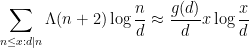
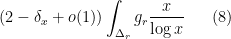
More generally, on the assumption of EH, the Bombieri asymptotic sieve provides the asymptotic

for any fixed 


is a further generalisation of the von Mangoldt function (now concentrated on 

![{\delta_x \in [0,2]}](https://s0.wp.com/latex.php?latex=%7B%5Cdelta_x+%5Cin+%5B0%2C2%5D%7D&bg=ffffff&fg=000000&s=0&c=20201002)


when 


and the twin prime conjecture would be proved if one could show that 


To put it another way, the Bombieri asymptotic sieve is able (on EH) to compute asymptotics for sums
without needing to know the unknown scalar 
for 


is obeyed (informally:
Because the obstruction to the parity problem is only one-dimensional (on EH), one can replace any parity-violating weight (such as

for some fixed 


where 


As it turns out, if one is willing to strengthen the assumption of the Elliott-Halberstam (EH) conjecture to the assumption of the generalised Elliott-Halberstam (GEH) conjecture (as formulated for instance in Claim 2.6 of the Polymath8b paper), one can also swap the 
in primes with 


for some fixed

of the Chowla conjecture, for which there has been some recent progress (discussed for instance in these recent posts). Informally, the Bombieri asymptotic sieve lets us (on GEH) view the twin prime conjecture as a sort of Chowla conjecture restricted to almost primes. Unfortunately, the recent progress on the Chowla conjecture relies heavily on the multiplicativity of
The Bombieri asymptotic sieve is already well explained in the original two papers of Bombieri; there is also a slightly different treatment of the sieve by Friedlander and Iwaniec, as well as a simplified version in the book of Friedlander and Iwaniec (in which the distribution hypothesis is strengthened in order to shorten the arguments. I’ve decided though to write up my own notes on the sieve below the fold; this is primarily for my own benefit, but may be useful to some readers also. I largely follow the treatment of Bombieri, with the one idiosyncratic twist of replacing the usual “elementary” Selberg sieve with the “analytic” Selberg sieve used in particular in many of the breakthrough works in small gaps between primes; I prefer working with the latter due to its Fourier-analytic flavour.
— 1. Controlling generalised von Mangoldt sums —
To prove (5), we shall first generalise it, by replacing the sequence 
- (i) (Non-negativity) One has
for all
.
- (ii) (Crude size bound) One has
for all
is the divisor function.
- (iii) (Size) We have
for some constant
.
- (iv) (Elliott-Halberstam type conjecture) For any
, one has
where
for all primes
.

These axioms are a little bit stronger than what is actually needed to make the Bombieri asymptotic sieve work, but we will not attempt to work with the weakest possible axioms here.
We introduce the function

which is analytic for 

There are two model examples of data 


The main result of this section is then
Theorem 1 Let
be as above. Let
be a tuple of natural numbers (independent of
as
.
Note that this recovers (5) (on EH) as a special case.
We now begin the proof of this theorem. Henceforth we allow implied constants in the 


It will be convenient to replace the range 


from which the original claim follows by a routine summation argument. Observe from axiom (iv) and the triangle inequality that

for any 
Write 


This function is just 
 .
.Proof: We induct on 


Since 
We can write
In the region 


for 


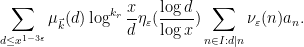
If we insert this replacement directly into the left-hand side of (10) and rearrange, we get

We can’t quite control this using axiom (iv) because the range of

where ![{\eta_\varepsilon: {\bf R} \rightarrow [0,1]}](https://s0.wp.com/latex.php?latex=%7B%5Ceta_%5Cvarepsilon%3A+%7B%5Cbf+R%7D+%5Crightarrow+%5B0%2C1%5D%7D&bg=ffffff&fg=000000&s=0&c=20201002)


where 


One could in principle compute 


which when compared with (14) for 

Inserting this back into (14) and recalling that
As it turns out, the estimate (13) is easy to establish, but the estimate (12) is not, roughly speaking because the typical number ![{[x^{1-4\varepsilon},1]}](https://s0.wp.com/latex.php?latex=%7B%5Bx%5E%7B1-4%5Cvarepsilon%7D%2C1%5D%7D&bg=ffffff&fg=000000&s=0&c=20201002)


for some quantity 

The key estimate is (16). As we shall see, when comparing 


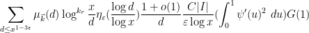
One has some flexibility in how to select the weight 


where ![{\psi: {\bf R} \rightarrow [0,1]}](https://s0.wp.com/latex.php?latex=%7B%5Cpsi%3A+%7B%5Cbf+R%7D+%5Crightarrow+%5B0%2C1%5D%7D&bg=ffffff&fg=000000&s=0&c=20201002)
![{[-1,1]}](https://s0.wp.com/latex.php?latex=%7B%5B-1%2C1%5D%7D&bg=ffffff&fg=000000&s=0&c=20201002)
![{[-1/2,1/2]}](https://s0.wp.com/latex.php?latex=%7B%5B-1%2F2%2C1%2F2%5D%7D&bg=ffffff&fg=000000&s=0&c=20201002)
It remains to establish the bounds (15), (16), (17). To warm up and introduce the various methods needed, we begin with the standard bound

where 

We now prove (19). The left-hand side can be expanded as
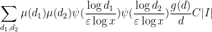
![\displaystyle \sum_{d_1,d_2} \mu(d_1) \mu(d_2) \psi( \frac{\log d_1}{\varepsilon \log x} ) \psi( \frac{\log d_2}{\varepsilon \log x} ) \sum_{n \in I: [d_1,d_2]|n} a_n](https://s0.wp.com/latex.php?latex=%5Cdisplaystyle+%5Csum_%7Bd_1%2Cd_2%7D+%5Cmu%28d_1%29+%5Cmu%28d_2%29+%5Cpsi%28+%5Cfrac%7B%5Clog+d_1%7D%7B%5Cvarepsilon+%5Clog+x%7D+%29+%5Cpsi%28+%5Cfrac%7B%5Clog+d_2%7D%7B%5Cvarepsilon+%5Clog+x%7D+%29+%5Csum_%7Bn+%5Cin+I%3A+%5Bd_1%2Cd_2%5D%7Cn%7D+a_n&bg=ffffff&fg=000000&s=0&c=20201002)
where ![{[d_1,d_2]}](https://s0.wp.com/latex.php?latex=%7B%5Bd_1%2Cd_2%5D%7D&bg=ffffff&fg=000000&s=0&c=20201002)
![{[d_1,d_2] \leq x^{2\varepsilon}}](https://s0.wp.com/latex.php?latex=%7B%5Bd_1%2Cd_2%5D+%5Cleq+x%5E%7B2%5Cvarepsilon%7D%7D&bg=ffffff&fg=000000&s=0&c=20201002)
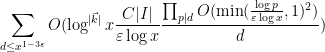
and an error term that is at most

From axiom (ii) and elementary multiplicative number theory, we have the bound

so from axiom (iv) and Cauchy-Schwarz we see that the error term (20) is acceptable. Thus it will suffice to establish the bound
![\displaystyle \sum_{d_1,d_2} \mu(d_1) \mu(d_2) \psi( \frac{\log d_1}{\varepsilon \log x} ) \psi( \frac{\log d_2}{\varepsilon \log x} ) \frac{g([d_1,d_2])}{[d_1,d_2]}](https://s0.wp.com/latex.php?latex=%5Cdisplaystyle+%5Csum_%7Bd_1%2Cd_2%7D+%5Cmu%28d_1%29+%5Cmu%28d_2%29+%5Cpsi%28+%5Cfrac%7B%5Clog+d_1%7D%7B%5Cvarepsilon+%5Clog+x%7D+%29+%5Cpsi%28+%5Cfrac%7B%5Clog+d_2%7D%7B%5Cvarepsilon+%5Clog+x%7D+%29+%5Cfrac%7Bg%28%5Bd_1%2Cd_2%5D%29%7D%7B%5Bd_1%2Cd_2%5D%7D+&bg=ffffff&fg=000000&s=0&c=20201002)

The summand here is almost, but not quite, multiplicative in 

for some rapidly decreasing function 


and so the left-hand side of (21) can be rearranged using Fubini’s theorem as

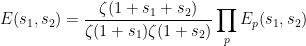
![\displaystyle E(s_1,s_2) := \sum_{d_1,d_2} \frac{\mu(d_1) \mu(d_2)}{d_1^{s_1}d_2^{s_2}} \frac{g([d_1,d_2])}{[d_1,d_2]}.](https://s0.wp.com/latex.php?latex=%5Cdisplaystyle+E%28s_1%2Cs_2%29+%3A%3D+%5Csum_%7Bd_1%2Cd_2%7D+%5Cfrac%7B%5Cmu%28d_1%29+%5Cmu%28d_2%29%7D%7Bd_1%5E%7Bs_1%7Dd_2%5E%7Bs_2%7D%7D+%5Cfrac%7Bg%28%5Bd_1%2Cd_2%5D%29%7D%7B%5Bd_1%2Cd_2%5D%7D.&bg=ffffff&fg=000000&s=0&c=20201002)
We can factorise 
Taking absolute values and using Mertens’ theorem leads to the crude bound

which when combined with the rapid decrease of 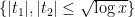

for
where

For 

and so by the Weierstrass 


we thus have

Also, since

and thus

The quantity (23) can thus be written, up to errors of 

Using the rapid decrease of 

But on differentiating and then squaring (22) we have

and the claim follows by integrating in 

We have the following variant of (19):
for any
. We also have the variant
If in addition
for some fixed
, one has
 , one has


Roughly speaking, the above estimates assert that
Proof: The left-hand side of (24) can be expanded as
![\displaystyle \sum_{d_1,d_2} \mu(d_1) \mu(d_2) \psi( \frac{\log d_1}{\varepsilon \log x} ) \psi( \frac{\log d_2}{\varepsilon \log x} ) \sum_{n \in I: [d_1,d_2,d]|n} a_n.](https://s0.wp.com/latex.php?latex=%5Cdisplaystyle+%5Csum_%7Bd_1%2Cd_2%7D+%5Cmu%28d_1%29+%5Cmu%28d_2%29+%5Cpsi%28+%5Cfrac%7B%5Clog+d_1%7D%7B%5Cvarepsilon+%5Clog+x%7D+%29+%5Cpsi%28+%5Cfrac%7B%5Clog+d_2%7D%7B%5Cvarepsilon+%5Clog+x%7D+%29+%5Csum_%7Bn+%5Cin+I%3A+%5Bd_1%2Cd_2%2Cd%5D%7Cn%7D+a_n.&bg=ffffff&fg=000000&s=0&c=20201002)
If we define

then the previous expression can be written as
![\displaystyle \sum_{d_1,d_2} \mu(d_1) \mu(d_2) \psi( \frac{\log d_1}{\varepsilon \log x} ) \psi( \frac{\log d_2}{\varepsilon \log x} ) \frac{g([d_1,d_2,d])}{[d_1,d_2,d]} C|I| + O(R_d),](https://s0.wp.com/latex.php?latex=%5Cdisplaystyle+%5Csum_%7Bd_1%2Cd_2%7D+%5Cmu%28d_1%29+%5Cmu%28d_2%29+%5Cpsi%28+%5Cfrac%7B%5Clog+d_1%7D%7B%5Cvarepsilon+%5Clog+x%7D+%29+%5Cpsi%28+%5Cfrac%7B%5Clog+d_2%7D%7B%5Cvarepsilon+%5Clog+x%7D+%29+%5Cfrac%7Bg%28%5Bd_1%2Cd_2%2Cd%5D%29%7D%7B%5Bd_1%2Cd_2%2Cd%5D%7D+C%7CI%7C+%2B+O%28R_d%29%2C&bg=ffffff&fg=000000&s=0&c=20201002)
while one has
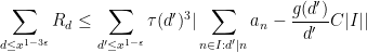
which gives (25) from Axiom (iv). To prove (24), it now suffices to show that
![\displaystyle \sum_{d_1,d_2} \mu(d_1) \mu(d_2) \psi( \frac{\log d_1}{\varepsilon \log x} ) \psi( \frac{\log d_2}{\varepsilon \log x} ) \frac{g([d_1,d_2,d])}{[d_1,d_2,d]}](https://s0.wp.com/latex.php?latex=%5Cdisplaystyle+%5Csum_%7Bd_1%2Cd_2%7D+%5Cmu%28d_1%29+%5Cmu%28d_2%29+%5Cpsi%28+%5Cfrac%7B%5Clog+d_1%7D%7B%5Cvarepsilon+%5Clog+x%7D+%29+%5Cpsi%28+%5Cfrac%7B%5Clog+d_2%7D%7B%5Cvarepsilon+%5Clog+x%7D+%29+%5Cfrac%7Bg%28%5Bd_1%2Cd_2%2Cd%5D%29%7D%7B%5Bd_1%2Cd_2%2Cd%5D%7D+&bg=ffffff&fg=000000&s=0&c=20201002)

Arguing as before, the left-hand side is

where
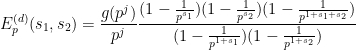
![\displaystyle E^{(d)}(s_1,s_2) := \sum_{d_1,d_2} \frac{\mu(d_1) \mu(d_2)}{d_1^{s_1}d_2^{s_2}} \frac{g([d_1,d_2,d])}{[d_1,d_2,d]}.](https://s0.wp.com/latex.php?latex=%5Cdisplaystyle+E%5E%7B%28d%29%7D%28s_1%2Cs_2%29+%3A%3D+%5Csum_%7Bd_1%2Cd_2%7D+%5Cfrac%7B%5Cmu%28d_1%29+%5Cmu%28d_2%29%7D%7Bd_1%5E%7Bs_1%7Dd_2%5E%7Bs_2%7D%7D+%5Cfrac%7Bg%28%5Bd_1%2Cd_2%2Cd%5D%29%7D%7B%5Bd_1%2Cd_2%2Cd%5D%7D.&bg=ffffff&fg=000000&s=0&c=20201002)
From Mertens’ theorem we have
when 


where 
if

and the claim (28) follows. When 

and (27) follows by repeating the previous calculations. Finally, (26) is proven similarly to (24) (using ![{d[d_1,d_2]}](https://s0.wp.com/latex.php?latex=%7Bd%5Bd_1%2Cd_2%5D%7D&bg=ffffff&fg=000000&s=0&c=20201002)
![{[d_1,d_2,d]}](https://s0.wp.com/latex.php?latex=%7B%5Bd_1%2Cd_2%2Cd%5D%7D&bg=ffffff&fg=000000&s=0&c=20201002)
Now we can prove (15), (16), (17). We begin with (15). Using the Leibniz rule 


Next, by applying the Leibniz rule to 


and hence we have the recursive identity

In particular, from induction we see that 

If 


- (a)
.
- (b)
.
The contribution of case (a) is easily seen to be acceptable by axiom (ii). For case (b), we observe from (30) and induction that
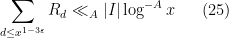
and so it will suffice to show that

where 


so by (25) it suffices to show that
subject to the same constraints on

applying Mertens’ theorem and summing over 
Now we show (16). As discussed previously in this section, we can replace

From the support of 


We can make the change of variables 

and then swap the sums to reduce to showing that
By Lemma 3, it suffices to show that
To prove this, we use the Rankin trick, bounding the implied weight 


which can be bounded by

and the claim follows from Mertens’ theorem.
Finally, we show (17). By (11), the left-hand side expands as
We let
plus a negligible error, where the 
up to negligible errors, where 


and so the total contribution of this case is 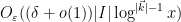
— 2. Weierstrass approximation —
Having proved Theorem 1, we now take linear combinations of this theorem, combined with the Weierstrass approximation theorem, to give the asymptotics (7), (8) described in the introduction.
Let 


whenever 
We now take a closer look at what happens when 

and hence

Multiplying by 

If we define

then an induction then shows that
for odd

for even
If we now define the comparison sequence 


for both odd and even
for any fixed
Next, from induction (on 


is a finite linear combination of functions of the form 


whenever 

where 


where now 


By linearity, this implies that


for any polynomial 


when
when


for any continuous function
Remark 4 The Bombieri asymptotic sieve has to use the full power of EH (or GEH); there are constructions due to Ford that show that if one only has a distributional hypothesis up to
for some fixed constant
, then the asymptotics of sums such as (5), or more generally (9), are not determined by a single scalar parameter
of distribution to be asymptotically equal to
, for which there is no consensus on what one should conjecturally expect.
The twin prime conjecture is one of the oldest unsolved problems in analytic number theory. There are several reasons why this conjecture remains out of reach of current techniques, but the most important obstacle is the parity problem which prevents purely sieve-theoretic methods (or many other popular methods in analytic number theory, such as the circle method) from detecting pairs of prime twins in a way that can distinguish them from other twins of almost primes. The parity problem is discussed in these previous blog posts; this obstruction is ultimately powered by the Möbius pseudorandomness principle that asserts that the Möbius function
However, there is an intriguing “alternate universe” in which the Möbius function is strongly correlated with some structured functions, and specifically with some Dirichlet characters, leading to the existence of the infamous “Siegel zero“. In this scenario, the parity problem obstruction disappears, and it becomes possible, in principle, to attack problems such as the twin prime conjecture. In particular, we have the following result of Heath-Brown:
Theorem 1 At least one of the following two statements are true:
- (Twin prime conjecture) There are infinitely many primes
- (No Siegel zeroes) There exists a constant
of conductor
, the associated Dirichlet
has no zeroes in the interval
.
Informally, this result asserts that if one had an infinite sequence of Siegel zeroes, one could use this to generate infinitely many twin primes. See this survey of Friedlander and Iwaniec for more on this “illusory” or “ghostly” parallel universe in analytic number theory that should not actually exist, but is surprisingly self-consistent and to date proven to be impossible to banish from the realm of possibility.
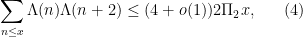
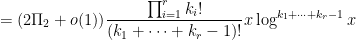
The strategy of Heath-Brown’s proof is fairly straightforward to describe. The usual starting point is to try to lower bound


 denotes Dirichlet convolution, and
  is an (unsquared) Selberg sieve that damps out small prime factors. This sum also detects twin primes, but will lead to slightly simpler computations. For technical reasons we will also smooth out the interval
  and remove very small primes from , but we will skip over these steps for the purpose of this informal discussion. (In Heath-Brown’s original paper, the Selberg sieve is essentially replaced by the more combinatorial restriction
  for some large , where
  is the primorial of
  , but I found the computations to be slightly easier if one works with a Selberg sieve, particularly if the sieve is not squared to make it nonnegative.)
If there is a Siegel zero 


The fact that ![{[x,2x]}](https://s0.wp.com/latex.php?latex=%7B%5Bx%2C2x%5D%7D&bg=ffffff&fg=000000&s=0&c=20201002)


 and the slowly varying function
  as being of about the same “complexity” as the constant function , so that
  is roughly of the same “complexity” as the divisor function
 to accuracy
  with little difficulty, whereas to obtain a comparable level of accuracy for
  or
or  is essentially the Riemann hypothesis.)
One expects 


 with
with  in various ranges; this is clearly related to understanding the equidistribution of the hyperbola
  in
in  . Taking Fourier transforms, the latter problem is closely related to estimation of the Kloosterman sums
 denotes the inverse of
  in
in  . One can then use the Weil bound
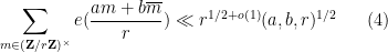
 is the greatest common divisor of
  (with the convention that this is equal to if
  vanish), and the decays to zero as
  . The Weil bound yields good enough control on error terms to estimate (3), and as it turns out the same method also works to estimate (2) (provided that
  with large enough).
Actually one does not need the full strength of the Weil bound here; any power savings over the trivial bound of
Lemma 2 (Kloosterman bound) One haswhenever

Proof: Observe from change of variables that the Kloosterman sum 


 has at most
  solutions
  to the system of equations
  . Hence the number of quadruples
  of the desired form is
  , and the claim follows.
We will also need another easy case of the Weil bound to handle some other portions of (2):
Lemma 3 (Easy Weil bound) Let. Then
Proof: As 


 . As is
  on the quadratic residues and
  on the non-residues, it now suffices to show that
 , the left-hand side becomes
  , and the claim follows.
While the basic strategy of Heath-Brown’s argument is relatively straightforward, implementing it requires a large amount of computation to control both main terms and error terms. I experimented for a while with rearranging the argument to try to reduce the amount of computation; I did not fully succeed in arriving at a satisfactorily minimal amount of superfluous calculation, but I was able to at least reduce this amount a bit, mostly by replacing a combinatorial sieve with a Selberg-type sieve (which was not needed to be positive, so I dispensed with the squaring aspect of the Selberg sieve to simplify the calculations a little further; also for minor reasons it was convenient to retain a tiny portion of the combinatorial sieve to eliminate extremely small primes). Also some modest reductions in complexity can be obtained by using the second von Mangoldt function 

We continue the discussion of sieve theory from Notes 4, but now specialise to the case of the linear sieve in which the sieve dimension 


for all primes 


for all square-free 


The fundamental lemma of sieve theory (Corollary 19 of Notes 4) gives us the bound

 is the quantity
This bound is strong when 


where we adopt the convention 

for all 
Exercise 1 (Alternate definition of
) Show that
is continuously differentiable except at
is continuously differentiable except at
where it is continuous, obeying the delay-differential equations
for
, with the initial conditions
for
and
for
. Show that these properties of


For future reference, we record the following explicit values of

 , and
, and 
for 
We will show
Theorem 2 (Linear sieve) Let the notation and hypotheses be as above, with
. Then, for any
, one has the upper bound
if
is sufficiently large depending on
. Furthermore, this claim is sharp in the sense that the quantity


Comparing the linear sieve with the fundamental lemma (and also testing using the sequence 


for all 
Exercise 3 Establish the integral identities
and
for
. Argue heuristically that these identities are consistent with the bounds in Theorem 2 and the Buchstab identity (Equation (16) from Notes 4).


Exercise 4 Use the Selberg sieve (Theorem 30 from Notes 4) to obtain a slightly weaker version of (12) in the range
in which the error term
is worsened to
, but the main term is unchanged.
We will prove Theorem 2 below the fold. The optimality of 


As an application of the linear sieve (specialised to the ranges in (10), (11)), we will establish a famous theorem of Chen, giving (in some sense) the closest approach to the twin prime conjecture that one can hope to achieve by sieve-theoretic methods:
Theorem 5 (Chen’s theorem) There are infinitely many primes
The same argument gives the version of Chen’s theorem for the even Goldbach conjecture, namely that for all sufficiently large even 

The discussion in these notes loosely follows that of Friedlander-Iwaniec (who study sieving problems in more general dimension than 

Recent Comments