
You are currently browsing the tag archive for the ‘time-frequency analysis’ tag.
This set of notes discusses aspects of one of the oldest questions in Fourier analysis, namely the nature of convergence of Fourier series.
If 

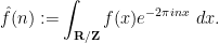
 is smooth, then the Fourier coefficients
  are absolutely summable, and we have the Fourier inversion formula
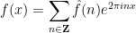
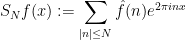
 converges uniformly to when is smooth.
What if 


Exercise 1
- (i) If
and
, show that
.)
- (ii) If
or
, show that there exists
The question of pointwise almost everywhere convergence turned out to be a significantly harder problem:
Theorem 2 (Pointwise almost everywhere convergence)
 such that
  is unbounded in
  ,
,  for almost every
  and
and
Note from Hölder’s inequality that 


Carleson’s theorem in particular was a surprisingly difficult result, lying just out of reach of classical methods (as we shall see later, the result is much easier if we smooth either the function
A recurring theme in mathematics is that of duality: a mathematical object 
- Vector space duality A vector space
over a field
can be described either by the set of vectors inside
from
). (If one is working in the category of topological vector spaces, one would work instead with continuous linear functionals; and so forth.) A fundamental connection between the two is given by the Hahn-Banach theorem (and its relatives).
- Vector subspace duality In a similar spirit, a subspace
of
. Again, the Hahn-Banach theorem provides a fundamental connection between the two perspectives.
- Convex duality More generally, a (closed, bounded) convex body
in a vector space
- Ideal-variety duality In a slightly different direction, an algebraic variety
can be viewed either “in physical space” or “internally” as a collection of points in
- Hilbert space duality An element
in a Hilbert space
can either be thought of in physical space as a vector in that space, or in momentum space as a covector
on that space. The fundamental connection between the two is given by the Riesz representation theorem for Hilbert spaces.
- Semantic-syntactic duality Much more generally still, a mathematical theory can either be described internally or syntactically via its axioms and theorems, or externally or semantically via its models. The fundamental connection between the two perspectives is given by the Gödel completeness theorem.
- Intrinsic-extrinsic duality A (Riemannian) manifold
can either be viewed intrinsically (using only concepts that do not require an ambient space, such as the Levi-Civita connection), or extrinsically, for instance as the level set of some defining function in an ambient space. Some important connections between the two perspectives includes the Nash embedding theorem and the theorema egregium.
- Group duality A group
can be described either via presentations (lists of generators, together with relations between them) or representations (realisations of that group in some more concrete group of transformations). A fundamental connection between the two is Cayley’s theorem. Unfortunately, in general it is difficult to build upon this connection (except in special cases, such as the abelian case), and one cannot always pass effortlessly from one perspective to the other.
- Pontryagin group duality A (locally compact Hausdorff) abelian group
, or by listing the characters
(i.e. continuous homomorphisms from
). The connection between the two is the focus of abstract harmonic analysis.
- Pontryagin subgroup duality A subgroup
. One of the fundamental connections between the two is the Poisson summation formula.
- Fourier duality A (sufficiently nice) function
on a locally compact abelian group
) can either be described in physical space (by its values
at each element
of
at elements
of the Pontryagin dual
- The uncertainty principle The behaviour of a function
is almost completely controlled by the behaviour of its Fourier transform
and vice versa, thanks to various mathematical manifestations of the uncertainty principle. (The Poisson summation formula can also be viewed as a variant of this principle, using subgroups instead of scales.)
- Stone/Gelfand duality A (locally compact Hausdorff) topological space
algebra
of continuous complex-valued functions on that space, or (in the case when
I have discussed a fair number of these examples in previous blog posts (indeed, most of the links above are to my own blog). In this post, I would like to discuss the uncertainty principle, that describes the dual relationship between physical space and frequency space. There are various concrete formalisations of this principle, most famously the Heisenberg uncertainty principle and the Hardy uncertainty principle – but in many situations, it is the heuristic formulation of the principle that is more useful and insightful than any particular rigorous theorem that attempts to capture that principle. Unfortunately, it is a bit tricky to formulate this heuristic in a succinct way that covers all the various applications of that principle; the Heisenberg inequality 
- A function which is band-limited (restricted to low frequencies) is featureless and smooth at fine scales, but can be oscillatory (i.e. containing plenty of cancellation) at coarse scales. Conversely, a function which is smooth at fine scales will be almost entirely restricted to low frequencies.
- A function which is restricted to high frequencies is oscillatory at fine scales, but is negligible at coarse scales. Conversely, a function which is oscillatory at fine scales will be almost entirely restricted to high frequencies.
- Projecting a function to low frequencies corresponds to averaging out (or spreading out) that function at fine scales, leaving only the coarse scale behaviour.
- Projecting a frequency to high frequencies corresponds to removing the averaged coarse scale behaviour, leaving only the fine scale oscillation.
- The number of degrees of freedom of a function is bounded by the product of its spatial uncertainty and its frequency uncertainty (or more generally, by the volume of the phase space uncertainty). In particular, there are not enough degrees of freedom for a non-trivial function to be simulatenously localised to both very fine scales and very low frequencies.
- To control the coarse scale (or global) averaged behaviour of a function, one essentially only needs to know the low frequency components of the function (and vice versa).
- To control the fine scale (or local) oscillation of a function, one only needs to know the high frequency components of the function (and vice versa).
- Localising a function to a region of physical space will cause its Fourier transform (or inverse Fourier transform) to resemble a plane wave on every dual region of frequency space.
- Averaging a function along certain spatial directions or at certain scales will cause the Fourier transform to become localised to the dual directions and scales. The smoother the averaging, the sharper the localisation.
- The smoother a function is, the more rapidly decreasing its Fourier transform (or inverse Fourier transform) is (and vice versa).
- If a function is smooth or almost constant in certain directions or at certain scales, then its Fourier transform (or inverse Fourier transform) will decay away from the dual directions or beyond the dual scales.
- If a function has a singularity spanning certain directions or certain scales, then its Fourier transform (or inverse Fourier transform) will decay slowly along the dual directions or within the dual scales.
- Localisation operations in position approximately commute with localisation operations in frequency so long as the product of the spatial uncertainty and the frequency uncertainty is significantly larger than one.
- In the high frequency (or large scale) limit, position and frequency asymptotically behave like a pair of classical observables, and partial differential equations asymptotically behave like classical ordinary differential equations. At lower frequencies (or finer scales), the former becomes a “quantum mechanical perturbation” of the latter, with the strength of the quantum effects increasing as one moves to increasingly lower frequencies and finer spatial scales.
- Etc., etc.
- Almost all of the above statements generalise to other locally compact abelian groups than
or
, in which the concept of a direction or scale is replaced by that of a subgroup or an approximate subgroup. (In particular, as we will see below, the Poisson summation formula can be viewed as another manifestation of the uncertainty principle.)
I think of all of the above (closely related) assertions as being instances of “the uncertainty principle”, but it seems difficult to combine them all into a single unified assertion, even at the heuristic level; they seem to be better arranged as a cloud of tightly interconnected assertions, each of which is reinforced by several of the others. The famous inequality
The uncertainty principle (as interpreted in the above broad sense) is one of the most fundamental principles in harmonic analysis (and more specifically, to the subfield of time-frequency analysis), second only to the Fourier inversion formula (and more generally, Plancherel’s theorem) in importance; understanding this principle is a key piece of intuition in the subject that one has to internalise before one can really get to grips with this subject (and also with closely related subjects, such as semi-classical analysis and microlocal analysis). Like many fundamental results in mathematics, the principle is not actually that difficult to understand, once one sees how it works; and when one needs to use it rigorously, it is usually not too difficult to improvise a suitable formalisation of the principle for the occasion. But, given how vague this principle is, it is difficult to present this principle in a traditional “theorem-proof-remark” manner. Even in the more informal format of a blog post, I was surprised by how challenging it was to describe my own understanding of this piece of mathematics in a linear fashion, despite (or perhaps because of) it being one of the most central and basic conceptual tools in my own personal mathematical toolbox. In the end, I chose to give below a cloud of interrelated discussions about this principle rather than a linear development of the theory, as this seemed to more closely align with the nature of this principle.
Camil Muscalu, Christoph Thiele and I have just uploaded to the arXiv our joint paper, “Multi-linear multipliers associated to simplexes of arbitrary length“, submitted to Analysis & PDE. This paper grew out of our project from many years ago to attempt to prove the nonlinear (or “scattering”) version of Carleson’s theorem on the almost everywhere convergence of Fourier series. This version is still open; our original approach was to handle the nonlinear Carleson operator by multilinear expansions in terms of the potential function V, but while the first three terms of this expansion were well behaved, the fourth term was unfortunately divergent, due to the unhelpful location of a certain minus sign. [This survey by Michael Lacey, as well as this paper of ourselves, covers some of these topics.]
However, what we did find out in this paper was that if we modified the nonlinear Carleson operator slightly, by replacing the underlying Schrödinger equation by a more general AKNS system, then for “generic” choices of this system, the problem of the ill-placed minus sign goes away, and each term in the multilinear series is, in fact, convergent (though we did not yet verify that the series actually converged, though in view of the earlier work of Christ and Kiselev on this topic, this seems likely). The verification of this convergence (at least with regard to the scattering data, rather than the more difficult analysis of the eigenfunctions) is the main result of our current paper. It builds upon our earlier estimates of the bilinear term in the expansion (which we dubbed the “biest”, as a multilingual pun). The main new idea in our earlier paper was to decompose the relevant region of frequency space 


A similar analysis happens to work for the multilinear operators associated to the frequency region 

(which generalises the bilinear Hilbert transform and the biest) obeys Hölder-type 

For the remainder of this post, I thought I would describe the “nonlinear Carleson theorem” conjecture, which is still one of my favourite open problems, being an excellent benchmark for measuring progress in the (still nascent) field of “nonlinear Fourier analysis“, while also being of interest in its own right in scattering and spectral theory.
Ciprian Demeter, Michael Lacey, Christoph Thiele and I have just uploaded our joint paper, “The Walsh model for 
Rather than discuss time-frequency analysis in detail here, I thought I would dwell instead on the return times theorem, and sketch how it is connected to the 
This is a well-known problem in multilinear harmonic analysis; it is fascinating to me because it lies barely beyond the reach of the best technology we have for these problems (namely, multiscale time-frequency analysis), and because the most recent developments in quadratic Fourier analysis seem likely to shed some light on this problem.
Recall that the Hilbert transform is defined on test functions 
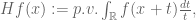
where the integral is evaluated in the principal value sense (removing the region 


Recent Comments