
You are currently browsing the category archive for the ‘math.AG’ category.
Louis Esser, Burt Totaro, Chengxi Wang, and myself have just uploaded to the arXiv our preprint “Varieties of general type with many vanishing plurigenera, and optimal sine and sawtooth inequalities“. This is an interdisciplinary paper that arose because in order to optimize a certain algebraic geometry construction it became necessary to solve a purely analytic question which, while simple, did not seem to have been previously studied in the literature. We were able to solve the analytic question exactly and thus fully optimize the algebraic geometry construction, though the analytic question may have some independent interest.
Let us first discuss the algebraic geometry application. Given a smooth complex 


 for some non-negative number
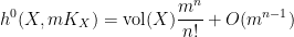
  , which is called the volume of the variety , which is an invariant that reveals some information about the birational geometry of . For instance, if the canonical line bundle is ample (or more generally, nef), this volume is equal to the intersection number
  (roughly speaking, the number of common zeroes of generic sections of the canonical line bundle); this is a special case of the asymptotic Riemann-Roch theorem. In particular, the volume is a natural number in this case. However, it is possible for the volume to also be fractional in nature. One can then ask: how small can the volume get without vanishing entirely? (By definition, varieties with non-vanishing volume are known as varieties of general type.)
It follows from a deep result obtained independently by Hacon–McKernan, Takayama and Tsuji that there is a uniform lower bound for the volume 


The space 


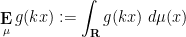
Now it is time to turn to the analytic side of the paper by describing the optimization problem that we solve. We consider the sawtooth function ![{g: {\bf R} \rightarrow (-1/2,1/2]}](https://s0.wp.com/latex.php?latex=%7Bg%3A+%7B%5Cbf+R%7D+%5Crightarrow+%28-1%2F2%2C1%2F2%5D%7D&bg=ffffff&fg=000000&s=0&c=20201002)

![{(-1/2,1/2]}](https://s0.wp.com/latex.php?latex=%7B%28-1%2F2%2C1%2F2%5D%7D&bg=ffffff&fg=000000&s=0&c=20201002)


 is bounded above by
  , we certainly have the trivial bound
 could attain the value of is if the probability measure was supported on half-integers, but in that case
  would vanish. For the algebraic geometry application discussed above one is then led to the following question: for a given choice of , what is the best upper bound
  on the quantity
 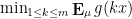 that holds for all probability measures ?
If one considers the deterministic case in which 


 . Thus we have
  is comparable to
  . In fact we were able to compute this quantity precisely:
Theorem 1 (Optimal bound for sawtooth inequality) Let.
In particular, we have
- (i) If
for some natural number
, then
.
- (ii) If
for some natural number
.
as
We establish this bound through duality. Indeed, suppose we could find non-negative coefficients 
 . Integrating this against an arbitrary probability measure , we would conclude
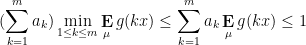
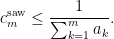 by selecting suitable candidate measures and computing the means
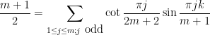
  . The theory of linear programming duality tells us that this method must give us the optimal bound, but one has to locate the optimal measure and optimal weights . This we were able to do by first doing some extensive numerics to discover these weights and measures for small values of , and then doing some educated guesswork to extrapolate these examples to the general case, and then to verify the required inequalities. In case (i) the situation is particularly simple, as one can take to be the discrete measure that assigns a probability
  to the numbers
  and the remaining probability of
  to
to  , while the optimal weighted inequality (1) turns out to be
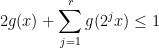
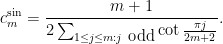
After solving the sawtooth problem, we became interested in the analogous question for the sine function, that is to say what is the best bound 
 Fourier coefficients of . To our knowledge this quantity has not previously been studied in the Fourier analysis literature. By adopting a similar approach as for the sawtooth problem, we were able to compute this quantity exactly also:
Theorem 2 For anyIn particular,
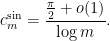
Interestingly, a closely related cotangent sum recently appeared in this MathOverflow post. Verifying the lower bound on 


 , first posed by Eisenstein in 1844 and proved by Stern in 1861. The upper bound arises from establishing the trigonometric inequality
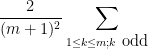
 , which to our knowledge is new; the left-hand side has a Fourier-analytic intepretation as convolving the Fejér kernel with a certain discretized square wave function, and this interpretation is used heavily in our proof of the inequality.
[UPDATE, Feb 1, 2021: the strategy sketched out below has been successfully implemented to rigorously obtain the desired implication in this recent preprint of Giulio Bresciani.]
I recently came across this question on MathOverflow asking if there are any polynomials 

On the other hand, the one surviving response to the question does point out this paper of Poonen which shows that assuming a powerful conjecture in Diophantine geometry known as the Bombieri-Lang conjecture (discussed in this previous post), it is at least possible to exhibit polynomials
I believe that it should be possible to also rule out the existence of bijective polynomials
Here is how I imagine a Bombieri-Lang-powered resolution of this question should proceed (modulo a large number of unjustified and somewhat vague steps that I believe to be true but have not established rigorously). Suppose for contradiction that we have a bijective polynomial 

has infinitely many rational points; indeed, every rational 


- (a) The rational points in
- (b) The rational points in
Consider case (b) first. By definition, this case asserts that the rational points in 


- (i) If
is birational to an elliptic curve, then the number of elements of
of height at most
should grow at most polylogarithmically in
.
- (ii) If
for some rational
, then then the number of elements of
(in fact I think it can only grow like
).
I do not have proofs of these results (though I think something similar to (i) can be found in Knapp’s book, and (ii) should basically follow by using a rational parameterisation 


for all 


for some rational functions 


This leaves the scenario in which case (a) holds for a “positive fraction” of 


Last week, we had Peter Scholze give an interesting distinguished lecture series here at UCLA on “Prismatic Cohomology”, which is a new type of cohomology theory worked out by Scholze and Bhargav Bhatt. (Video of the talks will be available shortly; for now we have some notes taken by two note–takers in the audience on that web page.) My understanding of this (speaking as someone that is rather far removed from this area) is that it is progress towards the “motivic” dream of being able to define cohomology 


- Singular cohomology, which roughly speaking works when the domain ring
or
, but can allow for arbitrary coefficients
- de Rham cohomology, which roughly speaking works as long as the coefficient ring
-adic cohomology, which is a remarkably powerful application of étale cohomology, but only works well when the coefficient ring
is localised around a prime
of the domain ring
- Crystalline cohomology, in which the domain ring is a field
of some finite characteristic
There are various relationships between the cohomology theories, for instance de Rham cohomology coincides with singular cohomology for smooth varieties in the limiting case 

The new prismatic cohomology of Bhatt and Scholze unifies many of these cohomologies in the “neighbourhood” of the point 


To define prismatic cohomology rings 


(And yes, Peter confirmed that he and Bhargav were inspired by the Dark Side of the Moon album cover in selecting the terminology.)
There was an abstract definition of prismatic cohomology (as being the essentially unique cohomology arising from prisms that obeyed certain natural axioms), but there was also a more concrete way to view them in terms of coordinates, as a “

prismatic cohomology in coordinates can be computed using a “
![\displaystyle d_q (t^n) = [n]_q t^{n-1} d_q t](https://s0.wp.com/latex.php?latex=%5Cdisplaystyle+d_q+%28t%5En%29+%3D+%5Bn%5D_q+t%5E%7Bn-1%7D+d_q+t&bg=ffffff&fg=000000&s=0&c=20201002)
where
![\displaystyle [n]_q = \frac{q^n-1}{q-1} = 1 + q + \dots + q^{n-1}](https://s0.wp.com/latex.php?latex=%5Cdisplaystyle+%5Bn%5D_q+%3D+%5Cfrac%7Bq%5En-1%7D%7Bq-1%7D+%3D+1+%2B+q+%2B+%5Cdots+%2B+q%5E%7Bn-1%7D&bg=ffffff&fg=000000&s=0&c=20201002)
is the “
Let 


![{[E:k]}](https://s0.wp.com/latex.php?latex=%7B%5BE%3Ak%5D%7D&bg=ffffff&fg=000000&s=0&c=20201002)

Theorem 1 (Fundamental theorem of Galois theory) Let
- (i) If
is an intermediate field betwen
, and
is a subgroup of
- (ii) Conversely, if
; namely
- (iii) If
and
, then
if and only if
is a subgroup of
.
- (iv) If
is isomorphic to the quotient group
.
Example 2 Let
, and let
be the degree
Galois extension formed by adjoining a primitive
root of unity (that is to say,
(the invertible elements of the ring
). Amongst the intermediate fields, one has the cyclotomic fields of the form
where
and
of
modulo
Example 3 Let
be the field of rational functions of one indeterminate
be the field formed by adjoining an
to
. Then
corresponding to the field automorphism of
to
). The intermediate fields are of the form
where
and
There is an analogous Galois correspondence in the covering theory of manifolds. For simplicity we restrict attention to finite covers. If 


Suppose 


Theorem 4 (Fundamental theorem of covering spaces) Let
- (i) If
is a subgroup of
- (ii) Conversely, if
.
- (iii) If
and
, then
if and only if
is a subgroup of
.
- (iv) If
is isomorphic to the quotient group
.
Example 5 Let
, and let
be the
. Then
with covering map
where
Given the strong similarity between the two theorems, it is natural to ask if there is some more concrete connection between Galois theory and the theory of finite covers.
In one direction, if the manifolds 


Exercise 6 What happens if one uses meromorphic functions in place of rational functions in the above example? (To answer this question, I found it convenient to use a discrete Fourier transform associated to the multiplicative action of the
of the coordinate
.)
I was curious however about the reverse direction. Starting with some field extensions 


The standard answer from modern algebraic geometry (as articulated for instance in this nice MathOverflow answer by Minhyong Kim) is to set 


![{{\bf C}[z, z^{-1}]}](https://s0.wp.com/latex.php?latex=%7B%7B%5Cbf+C%7D%5Bz%2C+z%5E%7B-1%7D%5D%7D&bg=ffffff&fg=000000&s=0&c=20201002)

![{\{ f \in {\bf C}[z, z^{-1}]: f(z_0)=0\}}](https://s0.wp.com/latex.php?latex=%7B%5C%7B+f+%5Cin+%7B%5Cbf+C%7D%5Bz%2C+z%5E%7B-1%7D%5D%3A+f%28z_0%29%3D0%5C%7D%7D&bg=ffffff&fg=000000&s=0&c=20201002)

![{\mathrm{Spec}( {\bf C}[z,z^{-1}] )}](https://s0.wp.com/latex.php?latex=%7B%5Cmathrm%7BSpec%7D%28+%7B%5Cbf+C%7D%5Bz%2Cz%5E%7B-1%7D%5D+%29%7D&bg=ffffff&fg=000000&s=0&c=20201002)
Of course, the spectrum of a field such as 

As an exercise, I set myself the task of trying to interpret Galois theory as an analogue of covering space theory in a more classical fashion, without explicit reference to more modern concepts such as schemes, spectra, or étale topology. After some experimentation, I found a reasonably satisfactory way to do so as follows. The space 


Below the fold I would like to record this interpretation of Galois theory, by first revisiting the theory of covering spaces using paths as the basic building block, and then adapting that theory to the theory of field extensions using the spaces indicated above. This is not too far from the usual scheme-theoretic way of phrasing the connection between the two topics (basically I have replaced étale-type points
Previous set of notes: 246B Notes 4. Next set of notes: Notes 2.
The fundamental object of study in real differential geometry are the real manifolds: Hausdorff topological spaces 


In a similar fashion, the fundamental object of study in complex differential geometry are the complex manifolds, in which the model space is 

Definition 1 (Riemann surface) If
of
on
and their inverses are all holomorphic. A Riemann surface is a Hausdorff connected topological space
A mapfrom one Riemann surface
is holomorphic if the maps
are holomorphic for any charts
of an atlas of
Here are some basic examples of Riemann surfaces.
Example 2 (Quotients of
as the single chart for an atlas). Of course, maps
that are holomorphic in the usual sense will also be holomorphic in the sense of the above definition, and vice versa, so the notion of holomorphicity for Riemann surfaces is compatible with that of holomorphicity for complex maps. More generally, given any discrete additive subgroup
of
is a Riemann surface. There are an infinite number of possible atlases to use here; one such is to pick a sufficiently small neighbourhood
of the origin in
where
and
for all
. In particular, given any non-real complex number
, the complex torus
formed by quotienting
is a Riemann surface.
Example 3 Any open connected subset
, other than
Example 4 (Riemann sphere) The Riemann sphere
, as a topological manifold, is the one-point compactification of
and
, and give these two open sets the charts
and
defined by
for
,
for
, and
. This is a complex atlas since the
is holomorphic on
.
An alternate way of viewing the Riemann sphere is as the projective line. Topologically, this is the punctured complex plane
quotiented out by non-zero complex dilations, thus elements of this space are equivalence classes
with the usual quotient topology. One can cover this space by two open sets
and
and give these two open sets the charts
and
for
. This is a complex atlas, basically because
for
Exercise 5 Verify that the Riemann sphere is isomorphic (as a Riemann surface) to the projective line.
Example 6 (Smooth algebraic plane curves) Let
be a complex polynomial in three variables which is homogeneous of some degree
, thus
Define the complex projective plane
to be the punctured space
quotiented out by non-zero complex dilations, with the usual quotient topology. (There is another important topology to place here of fundamental importance in algebraic geometry, namely the Zariski topology, but we will ignore this topology here.) This is a compact space, whose elements are equivalence classes
. Inside this plane we can define the (projective, degree
this is well defined thanks to (1). It is easy to verify that
is a closed subset of
Suppose thatsuch that the four numbers
simultaneously vanish for
. (This looks like four constraints, but is in fact essentially just three, due to the Euler identity
that arises from differentiating (1) in
. The fact that nonsingularity implies irreducibility is another consequence of Bezout’s theorem, which is not proven here.) For instance, the polynomial
is irreducible but singular (there is a “cusp” singularity at
). With this hypothesis, we call the curve
Now supposeis a point in
non-zero, and then we can normalise
. Now one can think of
as an inhomogeneous polynomial in just two variables
, and by nondegeneracy we see that the gradient
is non-zero whenever
. By the (complexified) implicit function theorem, this ensures that the affine algebraic curve
is a Riemann surface in a neighbourhood of
; we leave this as an exercise. This can be used to give a coordinate chart for
. Similarly when

![\displaystyle Z(P) := \{ [z_1,z_2,z_3] \in \mathbf{CP}^2: P(z_1,z_2,z_3) = 0 \};](https://s0.wp.com/latex.php?latex=%5Cdisplaystyle+Z%28P%29+%3A%3D+%5C%7B+%5Bz_1%2Cz_2%2Cz_3%5D+%5Cin+%5Cmathbf%7BCP%7D%5E2%3A+P%28z_1%2Cz_2%2Cz_3%29+%3D+0+%5C%7D%3B&bg=ffffff&fg=000000&s=0&c=20201002)


Exercise 7 State and prove a complex version of the implicit function theorem that justifies the above claim that the charts in the above example form an atlas, and an algebraic curve associated to a non-singular polynomial is a Riemann surface.
- (i) Show that all (irreducible plane projective) algebraic curves of degree
- (ii) Show that all (irreducible plane projective) algebraic curves of degree
are isomorphic to the Riemann sphere. (Hint: to reduce computation, first use some linear algebra to reduce the homogeneous quadratic polynomial to a standard form, such as
or
.)
Exercise 9 If
are complex numbers, show that the projective cubic curve
is nonsingular if and only if the discriminant
is non-zero. (When this occurs, the curve is called an elliptic curve (in Weierstrass form), which is a fundamentally important example of a Riemann surface in many areas of mathematics, and number theory in particular. One can also define the discriminant for polynomials of higher degree, but we will not do so here.)
![\displaystyle \{ [z_1, z_2, z_3]: z_2^2 z_3 = z_1^3 + a z_1 z_3^2 + b z_3^3 \}](https://s0.wp.com/latex.php?latex=%5Cdisplaystyle+%5C%7B+%5Bz_1%2C+z_2%2C+z_3%5D%3A+z_2%5E2+z_3+%3D+z_1%5E3+%2B+a+z_1+z_3%5E2+%2B+b+z_3%5E3+%5C%7D&bg=ffffff&fg=000000&s=0&c=20201002)
A recurring theme in mathematics is that an object
Definition 10 Let
. A meromorphic function on
; the space of all such functions will be denoted
.
One can also define holomorphicity and meromorphicity in terms of charts: a function 


On the complex numbers
It turns out, however, that the situation changes dramatically when the Riemann surface
Lemma 11 Let
be a holomorphic function on a compact Riemann surface
This result should be seen as a close sibling of Liouville’s theorem that all bounded entire functions are constant. (Indeed, in the case of a complex torus, this lemma is a corollary of Liouville’s theorem.)
Proof: As 

This dramatically cuts down the number of possible meromorphic functions – indeed, for an abstract Riemann surface, it is not immediately obvious that there are any non-constant meromorphic functions at all! As the poles are isolated and the surface is compact, a meromorphic function can only have finitely many poles, and if one prescribes the location of the poles and the maximum order at each pole, then we shall see that the space of meromorphic functions is now finite dimensional. The precise dimensions of these spaces are in fact rather interesting, and obey a basic duality law known as the Riemann-Roch theorem. We will give a mostly self-contained proof of the Riemann-Roch theorem in these notes, omitting only some facts about genus and Euler characteristic, as well as construction of certain meromorphic
A more detailed study of Riemann surface (and more generally, complex manifolds) can be found for instance in Griffiths and Harris’s “Principles of Algebraic Geometry“.
Read the rest of this entry »

In 1946, Ulam, in response to a theorem of Anning and Erdös, posed the following problem:
Problem 1 (Erdös-Ulam problem) Let
be a set such that the distance between any two points in
is rational. Is it true that
?
The paper of Anning and Erdös addressed the case that all the distances between two points in
The Erdös-Ulam problem remains open; it was discussed recently over at Gödel’s lost letter. It is in fact likely (as we shall see below) that the set
The main tool of the Solymosi-de Zeeuw analysis was Faltings’ celebrated theorem that every algebraic curve of genus at least two contains only finitely many rational points. The purpose of this post is to observe that an affirmative answer to the full Erdös-Ulam problem similarly follows from the conjectured analogue of Falting’s theorem for surfaces, namely the following conjecture of Bombieri and Lang:
Conjecture 2 (Bombieri-Lang conjecture) Let
which is of general type. Then the set
of rational points of
In fact, the Bombieri-Lang conjecture has been made for varieties of arbitrary dimension, and for more general number fields than the rationals, but the above special case of the conjecture is the only one needed for this application. We will review what “general type” means (for smooth projective complex varieties, at least) below the fold.
The Bombieri-Lang conjecture is considered to be extremely difficult, in particular being substantially harder than Faltings’ theorem, which is itself a highly non-trivial result. So this implication should not be viewed as a practical route to resolving the Erdös-Ulam problem unconditionally; rather, it is a demonstration of the power of the Bombieri-Lang conjecture. Still, it was an instructive algebraic geometry exercise for me to carry out the details of this implication, which quickly boils down to verifying that a certain quite explicit algebraic surface is of general type (Theorem 4 below). As I am not an expert in the subject, my computations here will be rather tedious and pedestrian; it is likely that they could be made much slicker by exploiting more of the machinery of modern algebraic geometry, and I would welcome any such streamlining by actual experts in this area. (For similar reasons, there may be more typos and errors than usual in this post; corrections are welcome as always.) My calculations here are based on a similar calculation of van Luijk, who used analogous arguments to show (assuming Bombieri-Lang) that the set of perfect cuboids is not Zariski-dense in its projective parameter space.
We also remark that in a recent paper of Makhul and Shaffaf, the Bombieri-Lang conjecture (or more precisely, a weaker consequence of that conjecture) was used to show that if
Let us now give the elementary reductions to the claim that a certain variety is of general type. For sake of contradiction, let 


Given any two points 


Now take four points 


for 


By inspecting the projection 


Claim 3 For any non-zero rational
in general position, the rational points of the affine surface
is not Zariski dense in
This is already very close to a claim that can be directly resolved by the Bombieri-Lang conjecture, but
![\displaystyle \overline{V} := \{ [X,Y,Z,R_1,R_2,R_3,R_4] \in {\bf CP}^6: Q(X,Y,Z,R_1,R_2,R_3,R_4) = 0 \} \ \ \ \ \ (1)](https://s0.wp.com/latex.php?latex=%5Cdisplaystyle+%5Coverline%7BV%7D+%3A%3D+%5C%7B+%5BX%2CY%2CZ%2CR_1%2CR_2%2CR_3%2CR_4%5D+%5Cin+%7B%5Cbf+CP%7D%5E6%3A+Q%28X%2CY%2CZ%2CR_1%2CR_2%2CR_3%2CR_4%29+%3D+0+%5C%7D+%5C+%5C+%5C+%5C+%5C+%281%29&bg=ffffff&fg=000000&s=0&c=20201002)
of 

with

and the projective complex space 
![{[X,Y,Z,R_1,R_2,R_3,R_4]}](https://s0.wp.com/latex.php?latex=%7B%5BX%2CY%2CZ%2CR_1%2CR_2%2CR_3%2CR_4%5D%7D&bg=ffffff&fg=000000&s=0&c=20201002)


![{\{ [X,Y,0,R_1,R_2,R_3,R_4]: X^2+bY^2=R^2; R_j = \pm R_1 \hbox{ for } j=2,3,4\}}](https://s0.wp.com/latex.php?latex=%7B%5C%7B+%5BX%2CY%2C0%2CR_1%2CR_2%2CR_3%2CR_4%5D%3A+X%5E2%2BbY%5E2%3DR%5E2%3B+R_j+%3D+%5Cpm+R_1+%5Chbox%7B+for+%7D+j%3D2%2C3%2C4%5C%7D%7D&bg=ffffff&fg=000000&s=0&c=20201002)
![{[X,Y,Z,R_1,R_2,R_3,R_4] \mapsto [X,Y,Z]}](https://s0.wp.com/latex.php?latex=%7B%5BX%2CY%2CZ%2CR_1%2CR_2%2CR_3%2CR_4%5D+%5Cmapsto+%5BX%2CY%2CZ%5D%7D&bg=ffffff&fg=000000&s=0&c=20201002)
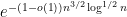
Heuristically, the reason why we expect few rational points in 


this is a convergent sum if
The Bombieri-Lang conjecture, Conjecture 2, can be viewed as a formalisation of the above heuristics (roughly speaking, it is one of the most optimistic natural conjectures one could make that is compatible with these heuristics while also being invariant under birational equivalence).
Unfortunately,

for 


![{[X,Y,Z]}](https://s0.wp.com/latex.php?latex=%7B%5BX%2CY%2CZ%5D%7D&bg=ffffff&fg=000000&s=0&c=20201002)
![{[x_j,y_j,1]}](https://s0.wp.com/latex.php?latex=%7B%5Bx_j%2Cy_j%2C1%5D%7D&bg=ffffff&fg=000000&s=0&c=20201002)


The other way in which could occur is if a non-trivial linear combination of at least two of the gradient vectors vanishes. From (2), this can only occur if 


for two choices of sign 


![\displaystyle [X,Y,Z,R_1,R_2,R_3,R_4] = [\pm \sqrt{b} i, 1, 0, 0, 0, 0, 0]. \ \ \ \ \ (5)](https://s0.wp.com/latex.php?latex=%5Cdisplaystyle+%5BX%2CY%2CZ%2CR_1%2CR_2%2CR_3%2CR_4%5D+%3D+%5B%5Cpm+%5Csqrt%7Bb%7D+i%2C+1%2C+0%2C+0%2C+0%2C+0%2C+0%5D.+%5C+%5C+%5C+%5C+%5C+%285%29&bg=ffffff&fg=000000&s=0&c=20201002)
If the non-trivial linear combination involved three or more gradient vectors, then by the pigeonhole principle at least two of the signs involved must be equal, and so the only singular points are (5). So the only remaining possibility is when we have two gradient vectors 


We will shortly show that the 

This will be done below the fold, by the pedestrian device of explicitly constructing global differential forms on
I thank Mark Green and David Gieseker for helpful conversations (and a crash course in varieties of general type!).
Remark 5 The above argument shows in fact (assuming Bombieri-Lang) that sets
, we obtain a similar conclusion with “rational” replaced by “lying in
Let 


![\displaystyle C = \{ [x,y,z]: y^2 z = x^3 + ax z^2 + b z^3 \}](https://s0.wp.com/latex.php?latex=%5Cdisplaystyle+C+%3D+%5C%7B+%5Bx%2Cy%2Cz%5D%3A+y%5E2+z+%3D+x%5E3+%2B+ax+z%5E2+%2B+b+z%5E3+%5C%7D&bg=ffffff&fg=000000&s=0&c=20201002)
in the projective plane ![{{\bf P}^2 = \{ [x,y,z]: (x,y,z) \neq (0,0,0) \}}](https://s0.wp.com/latex.php?latex=%7B%7B%5Cbf+P%7D%5E2+%3D+%5C%7B+%5Bx%2Cy%2Cz%5D%3A+%28x%2Cy%2Cz%29+%5Cneq+%280%2C0%2C0%29+%5C%7D%7D&bg=ffffff&fg=000000&s=0&c=20201002)


To each such curve 

 .
.The usual proofs of this bound proceed by first establishing a trace formula of the form

for some complex numbers 


In 1969, Stepanov introduced an elementary method (a version of what is now known as the polynomial method) to count (or at least to upper bound) the quantity
Theorem 2 (Weak Hasse-Weil bound) If
, then
.
In fact, the bound on
Theorem 2 is only an upper bound on 
I’ve discussed Bombieri’s proof of Theorem 2 in this previous post (in the special case of hyperelliptic curves), but now wish to present the full proof, with some minor simplifications from Bombieri’s original presentation; it is mostly elementary, with the deepest fact from algebraic geometry needed being Riemann’s inequality (a weak form of the Riemann-Roch theorem).
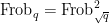
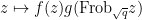
The first step is to reinterpret 

![\displaystyle \hbox{Frob}_q( [x_0,\dots,x_n] ) := [x_0^q, \dots, x_n^q]](https://s0.wp.com/latex.php?latex=%5Cdisplaystyle+%5Chbox%7BFrob%7D_q%28+%5Bx_0%2C%5Cdots%2Cx_n%5D+%29+%3A%3D+%5Bx_0%5Eq%2C+%5Cdots%2C+x_n%5Eq%5D&bg=ffffff&fg=000000&s=0&c=20201002)
then this map preserves the curve

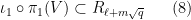
Thus one can interpret

and the Frobenius graph

which are copies of
with 


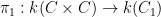
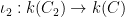
Let 


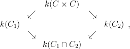
if we ignore the issue that a rational function on, say, 


The idea now is to find a rational function 


To find this
Now we build 

For any natural number 


For higher 

The former inequality just comes from the trivial inclusion 


From (3) and induction we see that each of the

Riemann’s inequality complements this with the lower bound

thus one has 


At any rate, now that we have these vector spaces 

for some natural numbers 


Observe that 

and in particular by (4)


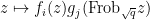
We will choose 


(together with (7)) then
On the other hand, we have the following basic fact:

 is injective.
Proof: From (3), we can find a linear basis 


This gives us the following bound:
Proposition 4 Let
be natural numbers such that (7), (11), (12) hold. Then
.
Proof: As 


If
and a brief calculation then gives Theorem 2. In some cases one can optimise things a bit further. For instance, in the genus zero case 


Remark 1 When
is not a perfect square, one can try to run the above argument using the factorisation
instead of
. This gives a weaker version of the above bound, of the shape
. In the hyperelliptic case at least, one can erase this loss by working with a variant of the argument in which one requires
Let 


The surface 


for all 

 , or equivalently that
for 

Theorem 1 (Monge-Cayley-Salmon theorem) Let
non-empty. Suppose that a Zariski dense set of points in
Among other things, this theorem was used in the celebrated result of Guth and Katz that almost solved the Erdos distance problem in two dimensions, as discussed in this previous blog post. Vanishing to third order is necessary: observe that in a surface of negative curvature, such as the saddle 
The original proof of the Monge-Cayley-Salmon theorem is not easily accessible and not written in modern language. A modern proof of this theorem (together with substantial generalisations, for instance to higher dimensions) is given by Landsberg; the proof uses the machinery of modern algebraic geometry. The purpose of this post is to record an alternate proof of the Monge-Cayley-Salmon theorem based on classical differential geometry (in particular, the notion of torsion of a curve) and basic ODE methods (in particular, Gronwall’s inequality and the Picard existence theorem). The idea is to “integrate” the lines 
Update: Janos Kollar has informed me that the above theorem was essentially known to Monge in 1809; see his recent arXiv note for more details.
I thank Larry Guth and Micha Sharir for conversations leading to this post.
The classical foundations of probability theory (discussed for instance in this previous blog post) is founded on the notion of a probability space 


![{{\bf P}: {\cal E} \rightarrow [0,1]}](https://s0.wp.com/latex.php?latex=%7B%7B%5Cbf+P%7D%3A+%7B%5Ccal+E%7D+%5Crightarrow+%5B0%2C1%5D%7D&bg=ffffff&fg=000000&s=0&c=20201002)
![{[0,1]}](https://s0.wp.com/latex.php?latex=%7B%5B0%2C1%5D%7D&bg=ffffff&fg=000000&s=0&c=20201002)
One can generalise the concept of a probability space to a finitely additive probability space, in which the event space 

In this post I would like to describe a further weakening of probability theory, which I will call qualitative probability theory, in which one does not assign a precise numerical probability value 


The main reason I want to introduce this weak notion of probability theory is that it becomes suited to talk about random variables living inside algebraic varieties, even if these varieties are defined over fields other than 


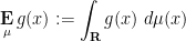
It turns out that just as qualitative random variables may be used to interpret the concept of a generic point, they can also be used to interpret the concept of a type in model theory; the type of a random variable 
Let

where 


is definable over
If 


In a recent paper, I established (in the large characteristic case) the following regularity lemma for dense definable graphs, which significantly strengthens the Szemerédi regularity lemma in this context, by eliminating “bad” pairs, giving a polynomially strong regularity, and also giving definability of the cells:
Lemma 1 (Algebraic regularity lemma) Let
be definable non-empty sets of complexity at most
also be definable with complexity at most
and
with
, with the following properties:
- (Definability) Each of the
are definable of complexity
.
- (Size) We have
and
for all
and
.
- (Regularity) We have
for all
, and
, where
is a rational number in

My original proof of this lemma was quite complicated, based on an explicit calculation of the “square”

of
Recently, Anand Pillay and Sergei Starchenko (and independently, Udi Hrushovski) have observed that the theory of the étale fundamental group is not necessary in the argument, and the lemma can in fact be deduced from quite general model theoretic techniques, in particular using (a local version of) the concept of stability. One of the consequences of this new proof of the lemma is that the hypothesis of large characteristic can be omitted; the lemma is now known to be valid for arbitrary finite fields
Inspired by this, I decided to see if I could find yet another proof of the algebraic regularity lemma, again avoiding the theory of the étale fundamental group. It turns out that the spectral proof of the Szemerédi regularity lemma (discussed in this previous blog post) adapts very nicely to this setting. The key fact needed about definable sets over finite fields is that their cardinality takes on an essentially discrete set of values. More precisely, we have the following fundamental result of Chatzidakis, van den Dries, and Macintyre:
Proposition 2 Let
.
- (Discretised cardinality) If
where
is a natural number, and
is a positive rational number with numerator and denominator
.
- (Definable cardinality) Assume
is sufficiently large depending on
, and
can be viewed as a definable subset of
, then for each natural number
is definable with complexity
depends definably on


We will take this proposition as a black box; a proof can be obtained by combining the description of definable sets over pseudofinite fields (discussed in this previous post) with the Lang-Weil bound (discussed in this previous post). (The former fact is phrased using nonstandard analysis, but one can use standard compactness-and-contradiction arguments to convert such statements to statements in standard analysis, as discussed in this post.)
The above proposition places severe restrictions on the cardinality of definable sets; for instance, it shows that one cannot have a definable set of complexity at most 


- If
for some
, then (if
is sufficiently small depending on
.
- If
for some
and
.
It turns out that these self-improving properties can be applied to the coefficients of various matrices (basically powers of the adjacency matrix associated to

Recent Comments