van Kampen’s theorem via covering spaces

If is a connected topological manifold, and is a point in , the (topological) fundamental group of at is traditionally defined as the space of equivalence classes of loops starting and ending at , with two loops considered equivalent if they are homotopic to each other. (One can of course define the fundamental group for more general classes of topological spaces, such as locally path connected spaces, but we will stick with topological manifolds in order to avoid pathologies.) As the name suggests, it is one of the most basic topological invariants of a manifold, which among other things can be used to classify the covering spaces of that manifold. Indeed, given any such covering , the fundamental group acts (on the right) by monodromy on the fibre , and conversely given any discrete set with a right action of , one can find a covering space with that monodromy action (this can be done by “tensoring” the universal cover with the given action, as illustrated below the fold). In more category-theoretic terms: monodromy produces an equivalence of categories between the category of covers of , and the category of discrete -sets.

One of the basic tools used to compute fundamental groups is van Kampen’s theorem:

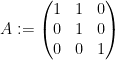
Theorem 1 (van Kampen’s theorem) Let be connected open sets covering a connected topological manifold with also connected, and let be an element of . Then is isomorphic to the amalgamated free product .

Since the topological fundamental group is customarily defined using loops, it is not surprising that many proofs of van Kampen’s theorem (e.g. the one in Hatcher’s text) proceed by an analysis of the loops in , carefully deforming them into combinations of loops in or in and using the combinatorial description of the amalgamated free product (which was discussed in this previous blog post). But I recently learned (thanks to the responses to this recent MathOverflow question of mine) that by using the above-mentioned equivalence of categories, one can convert statements about fundamental groups to statements about coverings. In particular, van Kampen’s theorem turns out to be equivalent to a basic statement about how to glue a cover of and a cover of together to give a cover of , and the amalgamated free product emerges through its categorical definition as a coproduct, rather than through its combinatorial description. One advantage of this alternate proof is that it can be extended to other contexts (such as the étale fundamental groups of varieties or schemes) in which the concept of a path or loop is no longer useful, but for which the notion of a covering is still important. I am thus recording (mostly for my own benefit) the covering-based proof of van Kampen’s theorem in the topological setting below the fold.

254A, Notes 5: The structure of locally compact groups, and Hilbert’s fifth problem

In the previous notes, we established the Gleason-Yamabe theorem:

Theorem 1 (Gleason-Yamabe theorem) Let be a locally compact group. Then, for any open neighbourhood of the identity, there exists an open subgroup of and a compact normal subgroup of in such that is isomorphic to a Lie group.

Roughly speaking, this theorem asserts the “mesoscopic” structure of a locally compact group (after restricting to an open subgroup to remove the macroscopic structure, and quotienting out by to remove the microscopic structure) is always of Lie type.

In this post, we combine the Gleason-Yamabe theorem with some additional tools from point-set topology to improve the description of locally compact groups in various situations.

We first record some easy special cases of this. If the locally compact group has the no small subgroups property, then one can take to be trivial; thus is Lie, which implies that is locally Lie and thus Lie as well. Thus the assertion that all locally compact NSS groups are Lie (Theorem 10 from Notes 4) is a special case of the Gleason-Yamabe theorem.

In a similar spirit, if the locally compact group is connected, then the only open subgroup of is the full group ; in particular, by arguing as in the treatment of the compact case (Exercise 19 of Notes 3), we conclude that any connected locally compact Hausdorff group is the inverse limit of Lie groups.

Now we return to the general case, in which need not be connected or NSS. One slight defect of Theorem 1 is that the group can depend on the open neighbourhood . However, by using a basic result from the theory of totally disconnected groups known as van Dantzig’s theorem, one can make independent of :

Theorem 2 (Gleason-Yamabe theorem, stronger version) Let be a locally compact group. Then there exists an open subgoup of such that, for any open neighbourhood of the identity in , there exists a compact normal subgroup of in such that is isomorphic to a Lie group.

We prove this theorem below the fold. As in previous notes, if is Hausdorff, the group is thus an inverse limit of Lie groups (and if (and hence ) is first countable, it is the inverse limit of a sequence of Lie groups).

It remains to analyse inverse limits of Lie groups. To do this, it helps to have some control on the dimensions of the Lie groups involved. A basic tool for this purpose is the invariance of domain theorem:

Theorem 3 (Brouwer invariance of domain theorem) Let be an open subset of , and let be a continuous injective map. Then is also open.

We prove this theorem below the fold. It has an important corollary:

Corollary 4 (Topological invariance of dimension) If , and is a non-empty open subset of , then there is no continuous injective mapping from to . In particular, and are not homeomorphic.

Exercise 1 (Uniqueness of dimension) Let be a non-empty topological space. If is a manifold of dimension , and also a manifold of dimension , show that . Thus, we may define the dimension of a non-empty manifold in a well-defined manner.

If are non-empty manifolds, and there is a continuous injection from to , show that .

Remark 1 Note that the analogue of the above exercise for surjections is false: the existence of a continuous surjection from one non-empty manifold to another does not imply that , thanks to the existence of space-filling curves. Thus we see that invariance of domain, while intuitively plausible, is not an entirely trivial observation.

As we shall see, we can use Corollary 4 to bound the dimension of the Lie groups in an inverse limit by the “dimension” of the inverse limit . Among other things, this can be used to obtain a positive resolution to Hilbert’s fifth problem:

Theorem 5 (Hilbert’s fifth problem) Every locally Euclidean group is isomorphic to a Lie group.

Again, this will be shown below the fold.

Another application of this machinery is the following variant of Hilbert’s fifth problem, which was used in Gromov’s original proof of Gromov’s theorem on groups of polynomial growth, although we will not actually need it this course:

Proposition 6 Let be a locally compact -compact group that acts transitively, faithfully, and continuously on a connected manifold . Then is isomorphic to a Lie group.

Recall that a continuous action of a topological group on a topological space is a continuous map which obeys the associativity law for and , and the identity law for all . The action is transitive if, for every , there is a with , and faithful if, whenever are distinct, one has for at least one .

The -compact hypothesis is a technical one, and can likely be dropped, but we retain it for this discussion (as in most applications we can reduce to this case).

Exercise 2 Show that Proposition 6 implies Theorem 5.

Remark 2 It is conjectured that the transitivity hypothesis in Proposition 6 can be dropped; this is known as the Hilbert-Smith conjecture. It remains open; the key difficulty is to figure out a way to eliminate the possibility that is a -adic group . See this previous blog post for further discussion.

254A, Notes 3: Haar measure and the Peter-Weyl theorem

In the last few notes, we have been steadily reducing the amount of regularity needed on a topological group in order to be able to show that it is in fact a Lie group, in the spirit of Hilbert’s fifth problem. Now, we will work on Hilbert’s fifth problem from the other end, starting with the minimal assumption of local compactness on a topological group , and seeing what kind of structures one can build using this assumption. (For simplicity we shall mostly confine our discussion to global groups rather than local groups for now.) In view of the preceding notes, we would like to see two types of structures emerge in particular:

• representations of into some more structured group, such as a matrix group ; and
• metrics on that capture the escape and commutator structure of (i.e. Gleason metrics).

To build either of these structures, a fundamentally useful tool is that of (left-) Haar measure – a left-invariant Radon measure on . (One can of course also consider right-Haar measures; in many cases (such as for compact or abelian groups), the two concepts are the same, but this is not always the case.) This concept generalises the concept of Lebesgue measure on Euclidean spaces , which is of course fundamental in analysis on those spaces.

Haar measures will help us build useful representations and useful metrics on locally compact groups . For instance, a Haar measure gives rise to the regular representation that maps each element of to the unitary translation operator on the Hilbert space of square-integrable measurable functions on with respect to this Haar measure by the formula

(The presence of the inverse is convenient in order to obtain the homomorphism property without a reversal in the group multiplication.) In general, this is an infinite-dimensional representation; but in many cases (and in particular, in the case when is compact) we can decompose this representation into a useful collection of finite-dimensional representations, leading to the Peter-Weyl theorem, which is a fundamental tool for understanding the structure of compact groups. This theorem is particularly simple in the compact abelian case, where it turns out that the representations can be decomposed into one-dimensional representations , better known as characters, leading to the theory of Fourier analysis on general compact abelian groups. With this and some additional (largely combinatorial) arguments, we will also be able to obtain satisfactory structural control on locally compact abelian groups as well.

The link between Haar measure and useful metrics on is a little more complicated. Firstly, once one has the regular representation , and given a suitable “test” function , one can then embed into (or into other function spaces on , such as or ) by mapping a group element to the translate of in that function space. (This map might not actually be an embedding if enjoys a non-trivial translation symmetry , but let us ignore this possibility for now.) One can then pull the metric structure on the function space back to a metric on , for instance defining an -based metric

if is square-integrable, or perhaps a -based metric

 

if is continuous and compactly supported (with denoting the supremum norm). These metrics tend to have several nice properties (for instance, they are automatically left-invariant), particularly if the test function is chosen to be sufficiently “smooth”. For instance, if we introduce the differentiation (or more precisely, finite difference) operators

(so that ) and use the metric (1), then a short computation (relying on the translation-invariance of the norm) shows that

for all . This suggests that commutator estimates, such as those appearing in the definition of a Gleason metric in Notes 2, might be available if one can control “second derivatives” of ; informally, we would like our test functions to have a “” type regularity.

If was already a Lie group (or something similar, such as a local group) then it would not be too difficult to concoct such a function by using local coordinates. But of course the whole point of Hilbert’s fifth problem is to do without such regularity hypotheses, and so we need to build test functions by other means. And here is where the Haar measure comes in: it provides the fundamental tool of convolution

between two suitable functions , which can be used to build smoother functions out of rougher ones. For instance:

Exercise 1 Let be continuous, compactly supported functions which are Lipschitz continuous. Show that the convolution using Lebesgue measure on obeys the -type commutator estimate

for all and some finite quantity depending only on .

This exercise suggests a strategy to build Gleason metrics by convolving together some “Lipschitz” test functions and then using the resulting convolution as a test function to define a metric. This strategy may seem somewhat circular because one needs a notion of metric in order to define Lipschitz continuity in the first place, but it turns out that the properties required on that metric are weaker than those that the Gleason metric will satisfy, and so one will be able to break the circularity by using a “bootstrap” or “induction” argument.

We will discuss this strategy – which is due to Gleason, and is fundamental to all currently known solutions to Hilbert’s fifth problem – in later posts. In this post, we will construct Haar measure on general locally compact groups, and then establish the Peter-Weyl theorem, which in turn can be used to obtain a reasonably satisfactory structural classification of both compact groups and locally compact abelian groups.

The inverse function theorem for everywhere differentiable maps

The classical inverse function theorem reads as follows:

Theorem 1 ( inverse function theorem) Let be an open set, and let be an continuously differentiable function, such that for every , the derivative map is invertible. Then is a local homeomorphism; thus, for every , there exists an open neighbourhood of and an open neighbourhood of such that is a homeomorphism from to .

It is also not difficult to show by inverting the Taylor expansion

that at each , the local inverses are also differentiable at with derivative

The textbook proof of the inverse function theorem proceeds by an application of the contraction mapping theorem. Indeed, one may normalise and to be the identity map; continuity of then shows that is close to the identity for small , which may be used (in conjunction with the fundamental theorem of calculus) to make a contraction on a small ball around the origin for small , at which point the contraction mapping theorem readily finishes off the problem.

I recently learned (after I asked this question on Math Overflow) that the hypothesis of continuous differentiability may be relaxed to just everywhere differentiability:

Theorem 2 (Everywhere differentiable inverse function theorem) Let be an open set, and let be an everywhere differentiable function, such that for every , the derivative map is invertible. Then is a local homeomorphism; thus, for every , there exists an open neighbourhood of and an open neighbourhood of such that is a homeomorphism from to .

As before, one can recover the differentiability of the local inverses, with the derivative of the inverse given by the usual formula (1).

This result implicitly follows from the more general results of Cernavskii about the structure of finite-to-one open and closed maps, however the arguments there are somewhat complicated (and subsequent proofs of those results, such as the one by Vaisala, use some powerful tools from algebraic geometry, such as dimension theory). There is however a more elementary proof of Saint Raymond that was pointed out to me by Julien Melleray. It only uses basic point-set topology (for instance, the concept of a connected component) and the basic topological and geometric structure of Euclidean space (in particular relying primarily on local compactness, local connectedness, and local convexity). I decided to present (an arrangement of) Saint Raymond’s proof here.

To obtain a local homeomorphism near , there are basically two things to show: local surjectivity near (thus, for near , one can solve for some near ) and local injectivity near (thus, for distinct near , is not equal to ). Local surjectivity is relatively easy; basically, the standard proof of the inverse function theorem works here, after replacing the contraction mapping theorem (which is no longer available due to the possibly discontinuous nature of ) with the Brouwer fixed point theorem instead (or one could also use degree theory, which is more or less an equivalent approach). The difficulty is local injectivity – one needs to preclude the existence of nearby points with ; note that in contrast to the contraction mapping theorem that provides both existence and uniqueness of fixed points, the Brouwer fixed point theorem only gives existence and not uniqueness.

In one dimension one can proceed by using Rolle’s theorem. Indeed, as one traverses the interval from to , one must encounter some intermediate point which maximises the quantity , and which is thus instantaneously non-increasing both to the left and to the right of . But, by hypothesis, is non-zero, and this easily leads to a contradiction.

Saint Raymond’s argument for the higher dimensional case proceeds in a broadly similar way. Starting with two nearby points with , one finds a point which “locally extremises” in the following sense: is equal to some , but is adherent to at least two distinct connected components of the set . (This is an oversimplification, as one has to restrict the available points in to a suitably small compact set, but let us ignore this technicality for now.) Note from the non-degenerate nature of that was already adherent to ; the point is that “disconnects” in some sense. Very roughly speaking, the way such a critical point is found is to look at the sets as shrinks from a large initial value down to zero, and one finds the first value of below which this set disconnects from . (Morally, one is performing some sort of Morse theory here on the function , though this function does not have anywhere near enough regularity for classical Morse theory to apply.)

The point is mapped to a point on the boundary of the ball , while the components are mapped to the interior of this ball. By using a continuity argument, one can show (again very roughly speaking) that must contain a “hemispherical” neighbourhood of inside , and similarly for . But then from differentiability of at , one can then show that and overlap near , giving a contradiction.

The rigorous details of the proof are provided below the fold.

254A, Notes 2: Building Lie structure from representations and metrics

Hilbert’s fifth problem concerns the minimal hypotheses one needs to place on a topological group to ensure that it is actually a Lie group. In the previous set of notes, we saw that one could reduce the regularity hypothesis imposed on to a “” condition, namely that there was an open neighbourhood of that was isomorphic (as a local group) to an open subset of a Euclidean space with identity element , and with group operation obeying the asymptotic

for sufficiently small . We will call such local groups local groups.

We now reduce the regularity hypothesis further, to one in which there is no explicit Euclidean space that is initially attached to . Of course, Lie groups are still locally Euclidean, so if the hypotheses on do not involve any explicit Euclidean spaces, then one must somehow build such spaces from other structures. One way to do so is to exploit an ambient space with Euclidean or Lie structure that is embedded or immersed in. A trivial example of this is provided by the following basic fact from linear algebra:

Lemma 1 If is a finite-dimensional vector space (i.e. it is isomorphic to for some ), and is a linear subspace of , then is also a finite-dimensional vector space.

We will establish a non-linear version of this statement, known as Cartan’s theorem. Recall that a subset of a -dimensional smooth manifold is a -dimensional smooth (embedded) submanifold of for some if for every point there is a smooth coordinate chart of a neighbourhood of in that maps to , such that , where we identify with a subspace of . Informally, locally sits inside the same way that sits inside .

Theorem 2 (Cartan’s theorem) If is a (topologically) closed subgroup of a Lie group , then is a smooth submanifold of , and is thus also a Lie group.

Note that the hypothesis that is closed is essential; for instance, the rationals are a subgroup of the (additive) group of reals , but the former is not a Lie group even though the latter is.

Exercise 1 Let be a subgroup of a locally compact group . Show that is closed in if and only if it is locally compact.

A variant of the above results is provided by using (faithful) representations instead of embeddings. Again, the linear version is trivial:

Lemma 3 If is a finite-dimensional vector space, and is another vector space with an injective linear transformation from to , then is also a finite-dimensional vector space.

Here is the non-linear version:

Theorem 4 (von Neumann’s theorem) If is a Lie group, and is a locally compact group with an injective continuous homomorphism , then also has the structure of a Lie group.

Actually, it will suffice for the homomorphism to be locally injective rather than injective; related to this, von Neumann’s theorem localises to the case when is a local group rather a group. The requirement that be locally compact is necessary, for much the same reason that the requirement that be closed was necessary in Cartan’s theorem.

Example 1 Let be the two-dimensional torus, let , and let be the map , where is a fixed real number. Then is a continuous homomorphism which is locally injective, and is even globally injective if is irrational, and so Theorem 4 is consistent with the fact that is a Lie group. On the other hand, note that when is irrational, then is not closed; and so Theorem 4 does not follow immediately from Theorem 2 in this case. (We will see, though, that Theorem 4 follows from a local version of Theorem 2.)

As a corollary of Theorem 4, we observe that any locally compact Hausdorff group with a faithful linear representation, i.e. a continuous injective homomorphism from into a linear group such as or , is necessarily a Lie group. This suggests a representation-theoretic approach to Hilbert’s fifth problem. While this approach does not seem to readily solve the entire problem, it can be used to establish a number of important special cases with a well-understood representation theory, such as the compact case or the abelian case (for which the requisite representation theory is given by the Peter-Weyl theorem and Pontryagin duality respectively). We will discuss these cases further in later notes.

In all of these cases, one is not really building up Euclidean or Lie structure completely from scratch, because there is already a Euclidean or Lie structure present in another object in the hypotheses. Now we turn to results that can create such structure assuming only what is ostensibly a weaker amount of structure. In the linear case, one example of this is is the following classical result in the theory of topological vector spaces.

Theorem 5 Let be a locally compact Hausdorff topological vector space. Then is isomorphic (as a topological vector space) to for some finite .

Remark 1 The Banach-Alaoglu theorem asserts that in a normed vector space , the closed unit ball in the dual space is always compact in the weak-* topology. Of course, this dual space may be infinite-dimensional. This however does not contradict the above theorem, because the closed unit ball is not a neighbourhood of the origin in the weak-* topology (it is only a neighbourhood with respect to the strong topology).

The full non-linear analogue of this theorem would be the Gleason-Yamabe theorem, which we are not yet ready to prove in this set of notes. However, by using methods similar to that used to prove Cartan’s theorem and von Neumann’s theorem, one can obtain a partial non-linear analogue which requires an additional hypothesis of a special type of metric, which we will call a Gleason metric:

Definition 6 Let be a topological group. A Gleason metric on is a left-invariant metric which generates the topology on and obeys the following properties for some constant , writing for :

• (Escape property) If and is such that , then .
• (Commutator estimate) If are such that , then

  

  where is the commutator of and .

Exercise 2 Let be a topological group that contains a neighbourhood of the identity isomorphic to a local group. Show that admits at least one Gleason metric.

Theorem 7 (Building Lie structure from Gleason metrics) Let be a locally compact group that has a Gleason metric. Then is isomorphic to a Lie group.

We will rely on Theorem 7 to solve Hilbert’s fifth problem; this theorem reduces the task of establishing Lie structure on a locally compact group to that of building a metric with suitable properties. Thus, much of the remainder of the solution of Hilbert’s fifth problem will now be focused on the problem of how to construct good metrics on a locally compact group.

In all of the above results, a key idea is to use one-parameter subgroups to convert from the nonlinear setting to the linear setting. Recall from the previous notes that in a Lie group , the one-parameter subgroups are in one-to-one correspondence with the elements of the Lie algebra , which is a vector space. In a general topological group , the concept of a one-parameter subgroup (i.e. a continuous homomorphism from to ) still makes sense; the main difficulties are then to show that the space of such subgroups continues to form a vector space, and that the associated exponential map is still a local homeomorphism near the origin.

Exercise 3 The purpose of this exercise is to illustrate the perspective that a topological group can be viewed as a non-linear analogue of a vector space. Let be locally compact groups. For technical reasons we assume that are both -compact and metrisable.

• (i) (Open mapping theorem) Show that if is a continuous homomorphism which is surjective, then it is open (i.e. the image of open sets is open). (Hint: mimic the proof of the open mapping theorem for Banach spaces, as discussed for instance in these notes. In particular, take advantage of the Baire category theorem.)
• (ii) (Closed graph theorem) Show that if a homomorphism is closed (i.e. its graph is a closed subset of ), then it is continuous. (Hint: mimic the derivation of the closed graph theorem from the open mapping theorem in the Banach space case, as again discussed in these notes.)
• (iii) Let be a homomorphism, and let be a continuous injective homomorphism into another Hausdorff topological group . Show that is continuous if and only if is continuous.
• (iv) Relax the condition of metrisability to that of being Hausdorff. (Hint: Now one cannot use the Baire category theorem for metric spaces; but there is an analogue of this theorem for locally compact Hausdorff spaces.)

Brouwer’s fixed point and invariance of domain theorems, and Hilbert’s fifth problem

We recall Brouwer’s famous fixed point theorem:

Theorem 1 (Brouwer fixed point theorem) Let be a continuous function on the unit ball in a Euclidean space . Then has at least one fixed point, thus there exists with .

This theorem has many proofs, most of which revolve (either explicitly or implicitly) around the notion of the degree of a continuous map of the unit sphere to itself, and more precisely around the stability of degree with respect to homotopy. (Indeed, one can view the Brouwer fixed point theorem as an assertion that some non-trivial degree-like invariant must exist, or more abstractly that the homotopy group is non-trivial.)

One of the many applications of this result is to prove Brouwer’s invariance of domain theorem:

Theorem 2 (Brouwer invariance of domain theorem) Let be an open subset of , and let be a continuous injective map. Then is also open.

This theorem in turn has an important corollary:

Corollary 3 (Topological invariance of dimension) If , and is a non-empty open subset of , then there is no continuous injective mapping from to . In particular, and are not homeomorphic.

This corollary is intuitively obvious, but note that topological intuition is not always rigorous. For instance, it is intuitively plausible that there should be no continuous surjection from to for , but such surjections always exist, thanks to variants of the Peano curve construction.

Theorem 2 or Corollary 3 can be proven by simple ad hoc means for small values of or (for instance, by noting that removing a point from will disconnect when , but not for ), but I do not know of any proof of these results in general dimension that does not require algebraic topology machinery that is at least as sophisticated as the Brouwer fixed point theorem. (Lebesgue, for instance, famously failed to establish the above corollary rigorously, although he did end up discovering the important concept of Lebesgue covering dimension as a result of his efforts.)

Nowadays, the invariance of domain theorem is usually proven using the machinery of singular homology. In this post I would like to record a short proof of Theorem 2 using Theorem 1 that I discovered in a paper of Kulpa, which avoids any use of algebraic topology tools beyond the fixed point theorem, though it is more ad hoc in its approach than the systematic singular homology approach.

Remark 1 A heuristic explanation as to why the Brouwer fixed point theorem is more or less a necessary ingredient in the proof of the invariance of domain theorem is that a counterexample to the former result could conceivably be used to create a counterexample to the latter one. Indeed, if the Brouwer fixed point theorem failed, then (as is well known) one would be able to find a continuous function that was the identity on (indeed, one could take to be the first point in which the ray from through hits ). If one then considered the function defined by , then this would be a continuous function which avoids the interior of , but which maps the origin to a point on the sphere (and maps to the dilate ). This could conceivably be a counterexample to Theorem 2, except that is not necessarily injective. I do not know if there is a more rigorous way to formulate this connection.

The reason I was looking for a proof of the invariance of domain theorem was that it comes up in the very last stage of the solution to Hilbert’s fifth problem, namely to establish the following fact:

Theorem 4 (Hilbert’s fifth problem) Every locally Euclidean group is isomorphic to a Lie group.

Recall that a locally Euclidean group is a topological group which is locally homeomorphic to an open subset of a Euclidean space , i.e. it is a continuous manifold. Note in contrast that a Lie group is a topological group which is locally diffeomorphic to an open subset of , it is a smooth manifold. Thus, Hilbert’s fifth problem is a manifestation of the “rigidity” of algebraic structure (in this case, group structure), which turns weak regularity (continuity) into strong regularity (smoothness).

It is plausible that something like Corollary 3 would need to be invoked in order to solve Hilbert’s fifth problem. After all, if Euclidean spaces , of different dimension were homeomorphic to each other, then the property of being locally Euclidean loses a lot of meaning, and would thus not be a particularly powerful hypothesis. Note also that it is clear that two Lie groups can only be isomorphic if they have the same dimension, so in view of Theorem 4, it becomes plausible that two Euclidean spaces can only be homeomorphic if they have the same dimension, although I do not know of a way to rigorously deduce this claim from Theorem 4.

Interestingly, Corollary 3 is the only place where algebraic topology enters into the solution of Hilbert’s fifth problem (although its cousin, point-set topology, is used all over the place). There are results closely related to Theorem 4, such as the Gleason-Yamabe theorem mentioned in a recent post, which do not use the notion of being locally Euclidean, and do not require algebraic topological methods in their proof. Indeed, one can deduce Theorem 4 from the Gleason-Yamabe theorem and invariance of domain; we sketch a proof of this (following Montgomery and Zippin) below the fold.

Central extensions of Lie groups, and cocycle averaging

In the last few months, I have been working my way through the theory behind the solution to Hilbert’s fifth problem, as I (together with Emmanuel Breuillard, Ben Green, and Tom Sanders) have found this theory to be useful in obtaining noncommutative inverse sumset theorems in arbitrary groups; I hope to be able to report on this connection at some later point on this blog. Among other things, this theory achieves the remarkable feat of creating a smooth Lie group structure out of what is ostensibly a much weaker structure, namely the structure of a locally compact group. The ability of algebraic structure (in this case, group structure) to upgrade weak regularity (in this case, continuous structure) to strong regularity (in this case, smooth and even analytic structure) seems to be a recurring theme in mathematics, and an important part of what I like to call the “dichotomy between structure and randomness”.

The theory of Hilbert’s fifth problem sprawls across many subfields of mathematics: Lie theory, representation theory, group theory, nonabelian Fourier analysis, point-set topology, and even a little bit of group cohomology. The latter aspect of this theory is what I want to focus on today. The general question that comes into play here is the extension problem: given two (topological or Lie) groups and , what is the structure of the possible groups that are formed by extending by . In other words, given a short exact sequence

to what extent is the structure of determined by that of and ?

As an example of why understanding the extension problem would help in structural theory, let us consider the task of classifying the structure of a Lie group . Firstly, we factor out the connected component of the identity as

as Lie groups are locally connected, is discrete. Thus, to understand general Lie groups, it suffices to understand the extensions of discrete groups by connected Lie groups.

Next, to study a connected Lie group , we can consider the conjugation action on the Lie algebra , which gives the adjoint representation . The kernel of this representation consists of all the group elements that commute with all elements of the Lie algebra, and thus (by connectedness) is the center of . The adjoint representation is then faithful on the quotient . The short exact sequence

then describes as a central extension (by the abelian Lie group ) of , which is a connected Lie group with a faithful finite-dimensional linear representation.

This suggests a route to Hilbert’s fifth problem, at least in the case of connected groups . Let be a connected locally compact group that we hope to demonstrate is isomorphic to a Lie group. As discussed in a previous post, we first form the space of one-parameter subgroups of (which should, eventually, become the Lie algebra of ). Hopefully, has the structure of a vector space. The group acts on by conjugation; this action should be both continuous and linear, giving an “adjoint representation” . The kernel of this representation should then be the center of . The quotient is locally compact and has a faithful linear representation, and is thus a Lie group by von Neumann’s version of Cartan’s theorem (discussed in this previous post). The group is locally compact abelian, and so it should be a relatively easy task to establish that it is also a Lie group. To finish the job, one needs the following result:

Theorem 1 (Central extensions of Lie are Lie) Let be a locally compact group which is a central extension of a Lie group by an abelian Lie group . Then is also isomorphic to a Lie group.

This result can be obtained by combining a result of Kuranishi with a result of Gleason; I am recording this argument below the fold. The point here is that while is initially only a topological group, the smooth structures of and can be combined (after a little bit of cohomology) to create the smooth structure on required to upgrade from a topological group to a Lie group. One of the main ideas here is to improve the behaviour of a cocycle by averaging it; this basic trick is helpful elsewhere in the theory, resolving a number of cohomological issues in topological group theory. The result can be generalised to show in fact that arbitrary (topological) extensions of Lie groups by Lie groups remain Lie; this was shown by Gleason. However, the above special case of this result is already sufficient (in conjunction with the rest of the theory, of course) to resolve Hilbert’s fifth problem.

Remark 1 We have shown in the above discussion that every connected Lie group is a central extension (by an abelian Lie group) of a Lie group with a faithful continuous linear representation. It is natural to ask whether this central extension is necessary. Unfortunately, not every connected Lie group admits a faithful continuous linear representation. An example (due to Birkhoff) is the Heisenberg-Weyl group

Indeed, if we consider the group elements

and

for some prime , then one easily verifies that has order and is central, and that is conjugate to . If we have a faithful linear representation of , then must have at least one eigenvalue that is a primitive root of unity. If is the eigenspace associated to , then must preserve , and be conjugate to on this space. This forces to have at least distinct eigenvalues on , and hence (and thus ) must have dimension at least . Letting we obtain a contradiction. (On the other hand, is certainly isomorphic to the extension of the linear group by the abelian group .)

van Dantzig’s theorem

This is yet another post in a series on basic ingredients in the structural theory of locally compact groups, which is closely related to Hilbert’s fifth problem.

In order to understand the structure of a topological group , a basic strategy is to try to split into two smaller factor groups by exhibiting a short exact sequence

If one has such a sequence, then is an extension of by (which includes direct products and semidirect products as examples, but can be more general than these situations, as discussed in this previous blog post). In principle, the problem of understanding the structure of then splits into three simpler problems:

1. (Horizontal structure) Understanding the structure of the “horizontal” group .
2. (Vertical structure) Understanding the structure of the “vertical” group .
3. (Cohomology) Understanding the ways in which one can extend by .

The “cohomological” aspect to this program can be nontrivial. However, in principle at least, this strategy reduces the study of the large group to the study of the smaller groups . (This type of splitting strategy is not restricted to topological groups, but can also be adapted to many other categories, particularly those of groups or group-like objects.) Typically, splitting alone does not fully kill off a structural classification problem, but it can reduce matters to studying those objects which are somehow “simple” or “irreducible”. For instance, this strategy can often be used to reduce questions about arbitrary finite groups to finite simple groups.

A simple example of splitting is as follows. Given any topological group , one can form the connected component of the identity – the maximal connected set containing the identity. It is not difficult to show that is a closed (and thus also locally compact) normal subgroup of , whose quotient is another locally compact group. Furthermore, due to the maximal connected nature of , is totally disconnected – the only connected sets are the singletons. In particular, is Hausdorff (the identity element is closed). Thus we have obtained a splitting

of an arbitrary locally compact group into a connected locally compact group , and a totally disconnected locally compact group . In principle at least, the study of locally compact groups thus splits into the study of connected locally compact groups, and the study of totally disconnected locally compact groups (though the cohomological issues are not always trivial).

In the structural theory of totally disconnected locally compact groups, the first basic theorem in the subject is van Dantzig’s theorem (which we prove below the fold):

Theorem 1 (Van Danztig’s theorem) Every totally disconnected locally compact group contains a compact open subgroup (which will of course still be totally disconnected).

Example 1 Let be a prime. Then the -adic field (with the usual -adic valuation) is totally disconnected locally compact, and the -adic integers are a compact open subgroup.

Of course, this situation is the polar opposite of what occurs in the connected case, in which the only open subgroup is the whole group.

In view of van Dantzig’s theorem, we see that the “local” behaviour of totally disconnected locally compact groups can be modeled by the compact totally disconnected groups, which are better understood (for instance, one can start analysing them using the Peter-Weyl theorem, as discussed in this previous post). The global behaviour however remains more complicated, in part because the compact open subgroup given by van Dantzig’s theorem need not be normal, and so does not necessarily induce a splitting of into compact and discrete factors.

Example 2 Let be a prime, and let be the semi-direct product , where the integers act on by the map , and we give the product of the discrete topology of and the -adic topology on . One easily verifies that is a totally disconnected locally compact group. It certainly has compact open subgroups, such as . However, it is easy to show that has no non-trivial compact normal subgroups (the problem is that the conjugation action of on has all non-trivial orbits unbounded).

Returning to more general locally compact groups, we obtain an immediate corollary:

Corollary 2 Every locally compact group contains an open subgroup which is “compact-by-connected” in the sense that is compact.

Indeed, one applies van Dantzig’s theorem to the totally disconnected group , and then pulls back the resulting compact open subgroup.

Now we mention another application of van Dantzig’s theorem, of more direct relevance to Hilbert’s fifth problem. Define a generalised Lie group to be a topological group with the property that given any open neighbourhood of the identity, there exists an open subgroup of and a compact normal subgroup of in such that is isomorphic to a Lie group. It is easy to see that such groups are locally compact. The deep Gleason-Yamabe theorem, which among other things establishes a satisfactory solution to Hilbert’s fifth problem (and which we will not prove here), asserts the converse:

Theorem 3 (Gleason-Yamabe theorem) Every locally compact group is a generalised Lie group.

Example 3 We consider the locally compact group from Example 2. This is of course not a Lie group. However, any open neighbourhood of the identity in will contain the compact subgroup for some integer . The open subgroup then has isomorphic to the discrete finite group , which is certainly a Lie group. Thus is a generalised Lie group.

One important example of generalised Lie groups are those locally compact groups which are an inverse limit (or projective limit) of Lie groups. Indeed, suppose we have a family of Lie groups indexed by partially ordered set which is directed in the sense that every finite subset of has an upper bound, together with continuous homomorphisms for all which form a category in the sense that for all . Then we can form the inverse limit

which is the subgroup of consisting of all tuples which are compatible with the in the sense that for all . If we endow with the product topology, then is a closed subgroup of , and thus has the structure of a topological group, with continuous homomorphisms which are compatible with the in the sense that for all . Such an inverse limit need not be locally compact; for instance, the inverse limit

of Euclidean spaces with the usual coordinate projection maps is isomorphic to the infinite product space with the product topology, which is not locally compact. However, if an inverse limit

of Lie groups is locally compact, it can be easily seen to be a generalised Lie group. Indeed, by local compactness, any open neighbourhood of the identity will contain an open precompact neighbourhood of the identity; by construction of the product topology (and the directed nature of ), this smaller neighbourhood will in turn will contain the kernel of one of the , which will be compact since the preceding neighbourhood was precompact. Quotienting out by this we obtain a locally compact subgroup of the Lie group , which is necessarily again a Lie group by Cartan’s theorem, and the claim follows.

In the converse direction, it is possible to use Corollary 2 to obtain the following observation of Gleason:

Theorem 4 Every Hausdorff generalised Lie group contains an open subgroup that is an inverse limit of Lie groups.

We show Theorem 4 below the fold. Combining this with the (substantially more difficult) Gleason-Yamabe theorem, we obtain quite a satisfactory description of the local structure of locally compact groups. (The situation is particularly simple for connected groups, which have no non-trivial open subgroups; we then conclude that every connected locally compact Hausdorff group is the inverse limit of Lie groups.)

Example 4 The locally compact group is not an inverse limit of Lie groups because (as noted earlier) it has no non-trivial compact normal subgroups, which would contradict the preceding analysis that showed that all locally compact inverse limits of Lie groups were generalised Lie groups. On the other hand, contains the open subgroup , which is the inverse limit of the discrete (and thus Lie) groups for (where we give the usual ordering, and use the obvious projection maps).

Locally compact groups with faithful finite-dimensional representations

This is another post in a series on various components to the solution of Hilbert’s fifth problem. One interpretation of this problem is to ask for a purely topological classification of the topological groups which are isomorphic to Lie groups. (Here we require Lie groups to be finite-dimensional, but allow them to be disconnected.)

There are some obvious necessary conditions on a topological group in order for it to be isomorphic to a Lie group; for instance, it must be Hausdorff and locally compact. These two conditions, by themselves, are not quite enough to force a Lie group structure; consider for instance a -adic field for some prime , which is a locally compact Hausdorff topological group which is not a Lie group (the topology is locally that of a Cantor set). Nevertheless, it turns out that by adding some key additional assumptions on the topological group, one can recover Lie structure. One such result, which is a key component of the full solution to Hilbert’s fifth problem, is the following result of von Neumann:

Theorem 1 Let be a locally compact Hausdorff topological group that has a faithful finite-dimensional linear representation, i.e. an injective continuous homomorphism into some linear group. Then can be given the structure of a Lie group. Furthermore, after giving this Lie structure, becomes smooth (and even analytic) and non-degenerate (the Jacobian always has full rank).

This result is closely related to a theorem of Cartan:

Theorem 2 (Cartan’s theorem) Any closed subgroup of a Lie group , is again a Lie group (in particular, is an analytic submanifold of , with the induced analytic structure).

Indeed, Theorem 1 immediately implies Theorem 2 in the important special case when the ambient Lie group is a linear group, and in any event it is not difficult to modify the proof of Theorem 1 to give a proof of Theorem 2. However, Theorem 1 is more general than Theorem 2 in some ways. For instance, let be the real line , which we faithfully represent in the -torus using an irrational embedding for some fixed irrational . The -torus can in turn be embedded in a linear group (e.g. by identifying it with , or ), thus giving a faithful linear representation of . However, the image is not closed (it is a dense subgroup of a -torus), and so Cartan’s theorem does not directly apply ( fails to be a Lie group). Nevertheless, Theorem 1 still applies and guarantees that the original group is a Lie group.

(On the other hand, the image of any compact subset of under a faithful representation must be closed, and so Theorem 1 is very close to the version of Theorem 2 for local groups.)

The key to building the Lie group structure on a topological group is to first build the associated Lie algebra structure, by means of one-parameter subgroups.

Definition 3 A one-parameter subgroup of a topological group is a continuous homomorphism from the real line (with the additive group structure) to .

Remark 1 Technically, is a parameterisation of a subgroup , rather than a subgroup itself, but we will abuse notation and refer to as the subgroup.

In a Lie group , the one-parameter subgroups are in one-to-one correspondence with the Lie algebra , with each element giving rise to a one-parameter subgroup , and conversely each one-parameter subgroup giving rise to an element of the Lie algebra; we will establish these basic facts in the special case of linear groups below the fold. On the other hand, the notion of a one-parameter subgroup can be defined in an arbitrary topological group. So this suggests the following strategy if one is to try to represent a topological group as a Lie group:

1. First, form the space of one-parameter subgroups of .
2. Show that has the structure of a (finite-dimensional) Lie algebra.
3. Show that “behaves like” the tangent space of at the identity (in particular, the one-parameter subgroups in should cover a neighbourhood of the identity in ).
4. Conclude that has the structure of a Lie group.

It turns out that this strategy indeed works to give Theorem 1 (and variants of this strategy are ubiquitious in the rest of the theory surrounding Hilbert’s fifth problem).

Below the fold, I record the proof of Theorem 1 (based on the exposition of Montgomery and Zippin). I plan to organise these disparate posts surrounding Hilbert’s fifth problem (and its application to related topics, such as Gromov’s theorem or to the classification of approximate groups) at a later date.

Locally compact topological vector spaces

Recall that a (real) topological vector space is a real vector space equipped with a topology that makes the vector space operations and continuous. One often restricts attention to Hausdorff topological vector spaces; in practice, this is not a severe restriction because it turns out that any topological vector space can be made Hausdorff by quotienting out the closure of the origin . One can also discuss complex topological vector spaces, and the theory is not significantly different; but for sake of exposition we shall restrict attention here to the real case.

An obvious example of a topological vector space is a finite-dimensional vector space such as with the usual topology. Of course, there are plenty of infinite-dimensional topological vector spaces also, such as infinite-dimensional normed vector spaces (with the strong, weak, or weak-* topologies) or Frechet spaces.

One way to distinguish the finite and infinite dimensional topological vector spaces is via local compactness. Recall that a topological space is locally compact if every point in that space has a compact neighbourhood. From the Heine-Borel theorem, all finite-dimensional vector spaces (with the usual topology) are locally compact. In infinite dimensions, one can trivially make a vector space locally compact by giving it a trivial topology, but once one restricts to the Hausdorff case, it seems impossible to make a space locally compact. For instance, in an infinite-dimensional normed vector space with the strong topology, an iteration of the Riesz lemma shows that the closed unit ball in that space contains an infinite sequence with no convergent subsequence, which (by the Heine-Borel theorem) implies that cannot be locally compact. If one gives the weak-* topology instead, then is now compact by the Banach-Alaoglu theorem, but is no longer a neighbourhood of the identity in this topology. In fact, we have the following result:

Theorem 1 Every locally compact Hausdorff topological vector space is finite-dimensional.

The first proof of this theorem that I am aware of is by André Weil. There is also a related result:

Theorem 2 Every finite-dimensional Hausdorff topological vector space has the usual topology.

As a corollary, every locally compact Hausdorff topological vector space is in fact isomorphic to with the usual topology for some . This can be viewed as a very special case of the theorem of Gleason, which is a key component of the solution to Hilbert’s fifth problem, that a locally compact group with no small subgroups (in the sense that there is a neighbourhood of the identity that contains no non-trivial subgroups) is necessarily isomorphic to a Lie group. Indeed, Theorem 1 is in fact used in the proof of Gleason’s theorem (the rough idea being to first locate a “tangent space” to at the origin, with the tangent vectors described by “one-parameter subgroups” of , and show that this space is a locally compact Hausdorff topological space, and hence finite dimensional by Theorem 1).

Theorem 2 may seem devoid of content, but it does contain some subtleties, as it hinges crucially on the joint continuity of the vector space operations and , and not just on the separate continuity in each coordinate. Consider for instance the one-dimensional vector space with the co-compact topology (a non-empty set is open iff its complement is compact in the usual topology). In this topology, the space is (though not Hausdorff), the scalar multiplication map is jointly continuous as long as the scalar is not zero, and the addition map is continuous in each coordinate (i.e. translations are continuous), but not jointly continuous; for instance, the set does not contain a non-trivial Cartesian product of two sets that are open in the co-compact topology. So this is not a counterexample to Theorem 2. Similarly for the cocountable or cofinite topologies on (the latter topology, incidentally, is the same as the Zariski topology on ).

Another near-counterexample comes from the topology of inherited by pulling back the usual topology on the unit circle . Admittedly, this pullback topology is not quite Hausdorff, but the addition map is jointly continuous. On the other hand, the scalar multiplication map is not continuous at all. A slight variant of this topology comes from pulling back the usual topology on the torus under the map for some irrational ; this restores the Hausdorff property, and addition is still jointly continuous, but multiplication remains discontinuous.

As some final examples, consider with the discrete topology; here, the topology is Hausdorff, addition is jointly continuous, and every dilation is continuous, but multiplication is not jointly continuous. If one instead gives the half-open topology, then again the topology is Hausdorff and addition is jointly continuous, but scalar multiplication is only jointly continuous once one restricts the scalar to be non-negative.

Below the fold, I record the textbook proof of Theorem 2 and Theorem 1. There is nothing particularly original in this presentation, but I wanted to record it here for my own future reference, and perhaps these results will also be of interest to some other readers.