
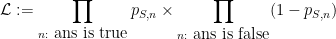
You are currently browsing the category archive for the ‘math.ST’ category.
This is a spinoff from the previous post. In that post, we remarked that whenever one receives a new piece of information 


 is the likelihood of this information under the alternative hypothesis , and
  is the likelihood of this information under the null hypothesis . If there are no other hypotheses under consideration, then the two posterior probabilities
  ,
,  must add up to one, and so can be recovered from the posterior odds
  by the formulae

A PDF version of the worksheet and instructions can be found here. One can fill in this worksheet in the following order:
- In Box 1, one enters in the precise statement of the null hypothesis
- In Box 2, one enters in the precise statement of the alternative hypothesis
- In Box 3, one enters in the prior probability
(or the best estimate thereof) of the null hypothesis
- In Box 4, one enters in the prior probability
(or the best estimate thereof) of the alternative hypothesis
.
- In Box 5, one enters in the ratio
between Box 4 and Box 3.
- In Box 6, one enters in the precise new information
- In Box 7, one enters in the likelihood
- In Box 8, one enters in the likelihood
- In Box 9, one enters in the ratio
betwen Box 8 and Box 7.
- In Box 10, one enters in the product of Box 5 and Box 9.
- (Assuming there are no other hypotheses than
divided by
- (Assuming there are no other hypotheses than
To illustrate this procedure, let us consider a standard Bayesian update problem. Suppose that a given point in time, 


We can fill out the entries in the worksheet one at a time:
- Box 1: The null hypothesis
- Box 2: The alternative hypothesis
- Box 3: In the absence of any better information, the prior probability
, or
.
- Box 4: Similarly, the prior probability
.
- Box 5: The prior odds
.
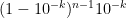
- Box 6: The new information
- Box 7: The likelihood
(the false positive rate).
- Box 8: The likelihood
, or
(one minus the false negative rate).
- Box 9: The likelihood ratio
.
- Box 10: The product of Box 5 and Box 9 is approximately
.
- Box 11: The posterior probability
is approximately
.
- Box 12: The posterior probability
is approximately
.
The filled worksheet looks like this:

Perhaps surprisingly, despite the positive COVID test, the employee 
We remark that if we switch the roles of the null hypothesis and alternative hypothesis, then some of the odds in the worksheet change, but the ultimate conclusions remain unchanged:

So the question of which hypothesis to designate as the null hypothesis and which one to designate as the alternative hypothesis is largely a matter of convention.
Now let us take a superficially similar situation in which a mother observers her daughter exhibiting COVID-like symptoms, to the point where she estimates the probability of her daughter having COVID at 
One can fill out the worksheet much as before, but now with the prior probability of the alternative hypothesis raised from 

Thus we see that prior probabilities can make a significant impact on the posterior probabilities.
Now we use the worksheet to analyze an infamous probability puzzle, the Monty Hall problem. Let us use the formulation given in that Wikipedia page:
Problem 1 Suppose you’re on a game show, and you’re given the choice of three doors: Behind one door is a car; behind the others, goats. You pick a door, say No. 1, and the host, who knows what’s behind the doors, opens another door, say No. 3, which has a goat. He then says to you, “Do you want to pick door No. 2?” Is it to your advantage to switch your choice?
For this problem, the precise formulation of the null hypothesis and the alternative hypothesis become rather important. Suppose we take the following two hypotheses:
- Null hypothesis
- Alternative hypothesis
 and
and  . The new information is that, after door 1 is selected, door 3 is revealed and shown to be a goat. After some thought, we conclude that is equal to
  (the host has a fifty-fifty chance of revealing door 3 instead of door 2) but that is also equal to (if the car is behind door 2, the host must reveal door 3, whereas if the car is behind door 3, the host cannot reveal door 3). Filling in the worksheet, we see that the new information does not in fact alter the odds, and the probability that the car is not behind door 1 remains at 2/3, so it is advantageous to switch.

However, consider the following different set of hypotheses:
- Null hypothesis
: The car is behind door number 1, and if you pick the door with the car, the host will reveal another door to entice you to switch. Otherwise, the host will not reveal a door.
- Alternative hypothesis
: The car is behind door number 2 or 3, and if you pick the door with the car, the host will reveal another door to entice you to switch. Otherwise, the host will not reveal a door.
Here we still have 


Finally, we consider another famous probability puzzle, the Sleeping Beauty problem. Again we quote the problem as formulated on the Wikipedia page:
Problem 2 Sleeping Beauty volunteers to undergo the following experiment and is told all of the following details: On Sunday she will be put to sleep. Once or twice, during the experiment, Sleeping Beauty will be awakened, interviewed, and put back to sleep with an amnesia-inducing drug that makes her forget that awakening. A fair coin will be tossed to determine which experimental procedure to undertake:Any time Sleeping Beauty is awakened and interviewed she will not be able to tell which day it is or whether she has been awakened before. During the interview Sleeping Beauty is asked: “What is your credence now for the proposition that the coin landed heads?”‘
- If the coin comes up heads, Sleeping Beauty will be awakened and interviewed on Monday only.
- If the coin comes up tails, she will be awakened and interviewed on Monday and Tuesday.
- In either case, she will be awakened on Wednesday without interview and the experiment ends.
Here the situation can be confusing because there are key portions of this experiment in which the observer is unconscious, but nevertheless Bayesian probability continues to operate regardless of whether the observer is conscious. To make this issue more precise, let us assume that the awakenings mentioned in the problem always occur at 8am, so in particular at 7am, Sleeping beauty will always be unconscious.
Here, the null and alternative hypotheses are easy to state precisely:
- Null hypothesis
- Alternative hypothesis
The subtle thing here is to work out what the correct prior state is (in most other applications of Bayesian probability, this state is obvious from the problem). It turns out that the most reasonable choice of prior state is “unconscious at 7am, on either Monday or Tuesday, with an equal chance of each”. (Note that whatever the outcome of the coin flip is, Sleeping Beauty will be unconscious at 7am Monday and unconscious again at 7am Tuesday, so it makes sense to give each of these two states an equal probability.) The new information is then
- New information
With this formulation, we see that 


There are arguments advanced in the literature to adopt the position that
If one has multiple pieces of information 
 is withheld from the person filling out the worksheet, for instance if that person relies exclusively on a news source that only reports information that supports the alternative hypothesis and omits information that debunks it, then the outcome of the worksheet is likely to be highly inaccurate, and one should only perform a Bayesian analysis when one has a high confidence that all relevant information (both favorable and unfavorable to the alternative hypothesis) is being reported to the user.
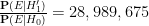
An unusual lottery result made the news recently: on October 1, 2022, the PCSO Grand Lotto in the Philippines, which draws six numbers from 

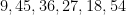


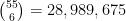
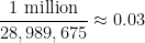
Whenever an event like this happens, journalists often contact mathematicians to ask the question: “What are the odds of this happening?”, and in fact I myself received one such inquiry this time around. This is a number that is not too difficult to compute – in this case, the probability of the lottery producing the six numbers 
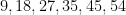
But on the previous draw of the same lottery, on September 28, 2022, the unremarkable sequence of numbers 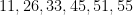

Part of the explanation surely lies in the unusually large number (
- The question “what are the odds of happening” is often easy to answer mathematically, but it is not the correct question to ask.
- The question “what is the probability that an alternative hypothesis is the truth” is (one of) the correct questions to ask, but is very difficult to answer (it involves both mathematical and non-mathematical considerations).
- The answer to the first question is one of the quantities needed to calculate the answer to the second, but it is far from the only such quantity. Most of the other quantities involved cannot be calculated exactly.
- However, by making some educated guesses, one can still sometimes get a very rough gauge of which events are “more surprising” than others, in that they would lead to relatively higher answers to the second question.
To explain these points it is convenient to adopt the framework of Bayesian probability. In this framework, one imagines that there are competing hypotheses to explain the world, and that one assigns a probability to each such hypothesis representing one’s belief in the truth of that hypothesis. For simplicity, let us assume that there are just two competing hypotheses to be entertained: the null hypothesis
- Null hypothesis
- Alternative hypothesis
At any given point in time, a person would have a probability 

Bayesian probability does not provide a rule for calculating the initial (or prior) probabilities 


What Bayesian probability does do, however, is provide a rule to update these probabilities 


 is the probability that the event would have occurred under the null hypothesis , and
  is the probability that the event would have occurred under the alternative hypothesis . Let us divide the second equation by the first to cancel the
  denominator, and obtain
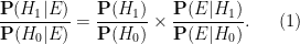
 as the prior odds of the alternative hypothesis, and
  as the posterior odds of the alternative hypothesis. The identity (1) then says that in order to compute the posterior odds
  of the alternative hypothesis in light of the new information , one needs to know three things:
- The prior odds
- The probability
- The probability
As previously discussed, the prior odds 

 . This is incredibly difficult to compute, because it requires a precise theory for how events would play out under the alternative hypothesis , and in particular is very sensitive as to what the alternative hypothesis actually is.
For instance, suppose we replace the alternative hypothesis
- Alternative hypothesis
, and views October 1 as their holiest day. On this day, they will manipulate the lottery to only select those balls that are multiples of
Under this alternative hypothesis 


Remark 1 The contrast between alternative hypothesis
At the opposite extreme, consider instead the following hypothesis:
- Alternative hypothesis
: The lottery is rigged by some corrupt officials, who on October 1 decide to randomly determine the winning numbers in advance, share these numbers with their collaborators, and then manipulate the lottery to choose those numbers that they selected.
If these corrupt officials are indeed choosing their predetermined winning numbers randomly, then the probability 
Now let us consider a third alternative hypothesis:
- Alternative hypothesis
: On October 1, the lottery machine developed a fault and now only selects numbers that exhibit unusual patterns.
Setting aside the question of precisely what faulty mechanism could induce this sort of effect, it is not clear at all how to compute 
 lottery outcomes that are “unusual”. Among such patterns would presumably be the multiples-of-9 pattern
  , but one could easily come up with other patterns that are equally “unusual”, such as consecutive strings such as
  , or the first few primes
  , or the first few squares
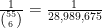
 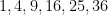 , and so forth. How many such unusual patterns are there? This is too vague a question to answer with any degree of precision, but as one illustrative statistic, the Online Encyclopedia of Integer Sequences (OEIS) currently hosts about
  sequences. Not all of these would begin with six distinct numbers from to , and several of these sequences might generate the same set of six numbers, but this does suggests that patterns that one would deem to be “unusual” could number in the thousands, tens of thousands, or more. Using this guess, we would then expect the event to boost the odds of this hypothesis by perhaps a thousandfold or so, which is moderately impressive. But subsequent information can counteract this effect. For instance, on October 3, the same lottery produced the numbers
  , which exhibit no unusual properties (no search results in the OEIS, for instance); if we denote this event by
  , then we have
 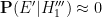 and so this new information should drive the odds for this alternative hypothesis way down again.
Remark 2 This example demonstrates another demagogical rhetorical technique that one sometimes sees (particularly in political or other emotionally charged contexts), which is to cherry-pick the information presented to their audience by informing them of eventsthat reported
Let us consider a superficially similar hypothesis:
- Alternative hypothesis
: On October 1, a divine being decided to send a sign to humanity by placing an unusual pattern in a lottery.
Here we (literally) stay agnostic on the prior odds of this hypothesis, and do not address the theological question of why a divine being should choose to use the medium of a lottery to send their signs. At first glance, the probability 

In summary, we have failed to locate any alternative hypothesis
- Has some non-negligible prior odds of being true (and in particular is not excessively specific, as with hypothesis
- Has a significantly higher probability of producing the specific event
- Does not struggle to also produce other events
; in the absence of these three factors, a moderately small numerical value of , such as does not actually do much to affect this plausibility. In this case one needs to lay out a reasonably precise alternative hypothesis and make some actual educated guesses towards the competing probability before one can lead to further conclusions. However, if is insanely small, e.g., less than  , then the possibility of a previously overlooked alternative hypothesis becomes far more plausible; as per the famous quote of Arthur Conan Doyle’s Sherlock Holmes, “When you have eliminated all which is impossible, then whatever remains, however improbable, must be the truth.”
We now return to the fact that for this specific October 1 lottery, there were 


- Null hypothesis
Then 
 draws or so), and standard probability theory suggests that the number of winners should now follow a Poisson distribution with this mean
  . The probability of obtaining winners would now be
  would be even smaller than this. So this clearly demands some sort of explanation. But in actuality, many purchasers of lottery tickets do not select their numbers completely randomly; they often have some “lucky” numbers (e.g., based on birthdays or other personally significant dates) that they prefer to use, or choose numbers according to a simple pattern rather than go to the trouble of trying to make them truly random. So if we modify the null hypothesis to
- Null hypothesis
: The lottery is run in a completely fair and random fashion, but a significant fraction of the purchasers of lottery tickets only select “unusual” numbers.
then it can now become quite plausible that a highly unusual set of numbers such as 

Remark 3 In view of the above discussion, one can propose a systematic way to evaluate (in as objective a fashion as possible) rhetorical claims in which an advocate is presenting evidence to support some alternative hypothesis:
- State the null hypothesis
- With the hypotheses precisely stated, give an honest estimate to the prior odds of this formulation of the alternative hypothesis.
- Consider if all the relevant information
- Estimate how likely the information
- Estimate how likely the information
- If the second estimate is significantly larger than the first, then you have cause to update your prior odds of this hypothesis (though if those prior odds were already vanishingly unlikely, this may not move the needle significantly). If not, the argument is unconvincing and no significant adjustment to the odds (except perhaps in a downwards direction) needs to be made.
In everyday usage, we rely heavily on percentages to quantify probabilities and proportions: we might say that a prediction is
- (i) In a two-party election, an outcome of say
to
might be considered close, but
to
would probably be viewed as a convincing mandate, and
to
would likely be viewed as a landslide.
- (ii) Similarly, if one were to poll an upcoming election, a poll of
- (iii) On the other hand, a medical operation that only had a
or
likely to be non-fatal (i.e., a
- (iv) A weather prediction of, say,
chance of rain during a vacation trip might be sufficient cause to pack an umbrella, even though it is more likely than not that rain would not occur. On the other hand, if the prediction was for an
- (v) Even extremely tiny percentages of toxic chemicals in everyday products can be considered unacceptable. For instance, EPA rules require action to be taken when the percentage of lead in drinking water exceeds
(15 parts per billion). At the opposite extreme, recycling contamination rates as high as
Because of all the very different ways in which percentages could be used, I think it may make sense to propose an alternate system of units to measure one class of probabilities, namely the probabilities of avoiding some highly undesirable outcome, such as death, accident or illness. The units I propose are that of “nines“, which are already commonly used to measure availability of some service or purity of a material, but can be equally used to measure the safety (i.e., lack of risk) of some activity. Informally, nines measure how many consecutive appearances of the digit
-
-
success = two nines of safety
-
success = three nines of safety
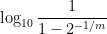
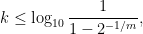
Definition 1 (Nines of safety) An activity (affecting one or more persons, over some given period of time) that has a probabilityof the “safe” outcome and probability
of the “unsafe” outcome will have
nines of safety against the unsafe outcome, where
(where
is the logarithm to base ten), or equivalently


Remark 2 Because of the various uncertainties in measuring probabilities, as well as the inaccuracies in some of the assumptions and approximations we will be making later, we will not attempt to measure the number of nines of safety beyond the first decimal point; thus we will round to the nearest tenth of a nine of safety throughout this post.
Here is a conversion table between percentage rates of success (the safe outcome), failure (the unsafe outcome), and the number of nines of safety one has:
| Success rate | Failure rate | Number of nines |
 |  |  |
| | |  |
 | |  |
| | |  |
| | |  |
| | |  |
 |  |  |
| | |  |
| | |  |
 |  |  |
 |  |  |
 |  |  |
| |  |  |
 |  |  |
 |  |  |
 |  |  |
 |  |  |
| | | infinite |
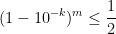
Thus, if one has no nines of safety whatsoever, one is guaranteed to fail; but each nine of safety one has reduces the failure rate by a factor of 
Remark 3 The number of nines of safety against a certain risk is not absolute; it will depend not only on the risk itself, but (a) the number of people exposed to the risk, and (b) the length of time one is exposed to the risk. Exposing more people or increasing the duration of exposure will reduce the number of nines, and conversely exposing fewer people or reducing the duration will increase the number of nines; see Proposition 7 below for a rough rule of thumb in this regard.
Remark 4 Nines of safety are a logarithmic scale of measurement, rather than a linear scale. Other familiar examples of logarithmic scales of measurement include the Richter scale of earthquake magnitude, the pH scale of acidity, the decibel scale of sound level, octaves in music, and the magnitude scale for stars.
Remark 5 One way to think about nines of safety is via the Swiss cheese model that was created recently to describe pandemic risk management. In this model, each nine of safety can be thought of as a slice of Swiss cheese, with holes occupying
Now to give some real-world examples of nines of safety. Using data for deaths in the US in 2019 (without attempting to account for factors such as age and gender), a random US citizen will have had the following amount of safety from dying from some selected causes in that year:
| Cause of death | Mortality rate per  (approx.) (approx.) | Nines of safety |
| All causes |  | |
| Heart disease |  | |
| Cancer |  | |
| Accidents |  | |
| Drug overdose |  | |
| Influenza/Pneumonia |  |  |
| Suicide |  | |
| Gun violence |  |  |
| Car accident |  | |
| Murder |  |  |
| Airplane crash |  |  |
| Lightning strike |  |  |
The safety of air travel is particularly remarkable: a given hour of flying in general aviation has a fatality rate of 


Of course, in 2020, COVID-19 deaths became significant. In this year in the US, the mortality rate for COVID-19 (as the underlying or contributing cause of death) was 
Some further illustrations of the concept of nines of safety:
- Each round of Russian roulette has a success rate of
, providing only
nines of safety after two rounds,
nines after three rounds, and so forth. (See also Proposition 7 below.)
- The ancient Roman punishment of decimation, by definition, provided exactly one nine of safety to each soldier being punished.
- Rolling a
-sided die is a risk that carries about
- Rolling a double one (“snake eyes“) from two six-sided dice carries about
- One has about
- A null hypothesis has
statistically significant result, and
statistically significant result. (However, one has to be careful when reversing the conditional; a
- If a poker opponent is dealt a five-card hand, one has
nines of safety against that opponent being dealt a royal flush,
against a straight flush or higher,
against a full house or higher,
against a flush or higher,
against a straight or higher,
against three-of-a-kind or higher,
against two pairs or higher, and just
- A
nines of safety against a single guess. (For the reduction in safety caused by multiple guesses, see Proposition 7 below.)
Here is another way to think about nines of safety:
Proposition 6 (Nines of safety extend expected onset of risk) Suppose a certain risky activity has.
Proof: The probability that the risk is activated after exactly 


Thus, for instance, if one performs some risky activity daily, then the expected length of time before the risk occurs is given by the following table:
| Daily nines of safety | Expected onset of risk |
 | One day |
| | One week |
| | One month |
| | One year |
 | Two years |
| | Five years |
| | Ten years |
| | Twenty years |
| | Fifty years |
 | A century |
Or, if one wants to convert the yearly risks of dying from a specific cause into expected years before that cause of death would occur (assuming for sake of discussion that no other cause of death exists):
| Yearly nines of safety | Expected onset of risk |
| | One year |
| | Two years |
| | Five years |
| | Ten years |
| | Twenty years |
| | Fifty years |
| | A century |
These tables suggest a relationship between the amount of safety one would have in a short timeframe, such as a day, and a longer time frame, such as a year. Here is an approximate formalisation of that relationship:
Proposition 7 (Repeated exposure reduces nines of safety) If a risky activity withtimes, then (assuming
nines of safety. Conversely: if the repeated activity has
nines of safety, the individual activity will have approximately
nines of safety.
Proof: An activity with 


Remark 8 The hypothesis of independence here is key. If there is a lot of correlation between the risks between different repetitions of the activity, then there can be much less reduction in safety caused by that repetition. As a simple example, suppose that; but in this case there is perfect correlation, and in fact the number of nines of safety remains steady at
Because of this caveat, one should view the above proposition as only a crude first approximation that can be used as a simple rule of thumb, but should not be relied upon for more precise calculations.
One can repeat a risk either in time (extending the time of exposure to the risk, say from a day to a year), or in space (by exposing the risk to more people). The above proposition then gives an additive conversion law for nines of safety in either case. Here are some conversion tables for time:
| From/to | Daily | Weekly | Monthly | Yearly |
| Daily | 0 | -0.8 | -1.5 | -2.6 |
| Weekly | +0.8 | 0 | -0.6 | -1.7 |
| Monthly | +1.5 | +0.6 | 0 | -1.1 |
| Yearly | +2.6 | +1.7 | +1.1 | 0 |
| From/to | Yearly | Per 5 yr | Per decade | Per century |
| Yearly | 0 | -0.7 | -1.0 | -2.0 |
| Per 5 yr | +0.7 | 0 | -0.3 | -1.3 |
| Per decade | +1.0 | + -0.3 | 0 | -1.0 |
| Per century | +2.0 | +1.3 | +1.0 | 0 |
For instance, as mentioned before, the yearly amount of safety against cancer is about 


Now we turn to conversions in space. If one knows the level of safety against a certain risk for an individual, and then one (independently) exposes a group of such individuals to that risk, then the reduction in nines of safety when considering the possibility that at least one group member experiences this risk is given by the following table:
| Group | Reduction in safety |
| You ( person) | |
You and your partner ( people) people) |  |
You and your parents ( people) people) |  |
| You, your partner, and three children ( people) |  |
| An extended family of people |  |
| A class of people |  |
A workplace of  people people |  |
A school of  people people |  |
A university of  people people |  |
| A town of people |  |
| A city of million people |  |
| A state of million people |  |
| A country of million people |  |
| A continent of billion people |  |
| The entire planet |  |
For instance, in a given year (and making the somewhat implausible assumption of independence), you might have 


In the opposite direction, any reduction in exposure (either in time or space) to a risk will increase one’s safety level, as per the following table:
| Reduction in exposure | Additional nines of safety |
 | |
 |  |
 |  |
 |  |
 |  |
 |  |
For instance, a five-fold reduction in exposure will reclaim about
Here is a slightly different way to view nines of safety:
Proposition 9 Suppose that a group ofnines of individual safety against that risk, then there is at least a
Proof: If individually there are
Thus, for a group to collectively avoid a risk with at least a
| Group | Individual safety level required |
| You ( person) | |
| You and your partner ( people) | |
| You and your parents ( people) | |
| You, your partner, and three children ( people) |  |
| An extended family of people |  |
| A class of people | |
| A workplace of people |  |
| A school of people |  |
| A university of people |  |
| A town of people |  |
| A city of million people |  |
| A state of million people | |
| A country of million people |  |
| A continent of billion people |  |
| The entire planet |  |
For large 
Precautions that can work to prevent a certain risk from occurring will add additional nines of safety against that risk, even if the precaution is not
Proposition 10 (Precautions add nines of safety) Suppose an activity carriesnines of safety (that is to say, the probability that the protection is effective is
). Then applying that precaution increases the number of nines in the activity from
.
Proof: The probability that the precaution fails and the risk then occurs is 
In particular, we can repurpose the table at the start of this post as a conversion chart for effectiveness of a precaution:
| Effectiveness | Failure rate | Additional nines provided |
| | |  |
| | | |
| | |  |
| | | |
| | | |
| | |  |
| | |  |
| | |  |
| | | |
| | |  |
| | |  |
| | |  |
| | |  |
| | |  |
| | |  |
| | |  |
| | |  |
| | | infinite |
Thus for instance a precaution that is 

A slight variant of the above rule can be stated using the concept of relative risk:
Proposition 11 (Relative risk and nines of safety) Suppose an activity carries. Then the action removes
nines of safety (if
) or adds
nines of safety (if
) to the original activity.
Proof: The additional action adjusts the probability of failure from 
Here is a conversion chart between relative risk and change in nines of safety:
| Relative risk | Change in nines of safety |
 | |
| | |
| | |
 | |
 | |
| | |
| | |
| | |
| | |
| | |
| |  |
 |  |
| | |
Some examples:
- Smoking increases the fatality rate of lung cancer by a factor of about
- Seatbelts reduce the fatality rate in car accidents by a factor of about two, adding about
, adding about
additional nines of safety.
- As far as transmission of COVID is concerned, it seems that constant use of face masks reduces transmission by a factor of about five (thus adding about
The effect of combining multiple (independent) precautions together is cumulative; one can achieve quite a high level of safety by stacking together several precautions that individually have relatively low levels of effectiveness. Again, see the “swiss cheese model” referred to in Remark 5. For instance, if face masks add
In summary, when debating the value of a given risk mitigation measure, the correct question to ask is not quite “Is it certain to work” or “Can it fail?”, but rather “How many extra nines of safety does it add?”.
As one final comparison between nines of safety and other standard risk measures, we give the following proposition regarding large deviations from the mean.
Proposition 12 Let, and let
. Then the “one-sided risk” of
by at least
(i.e.,
) carries
nines of safety, the “two-sided risk” of
) carries
nines of safety, where
is the error function.
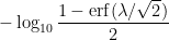
Proof: This is a routine calculation using the cumulative distribution function of the normal distribution.
Here is a short table illustrating this proposition:
Number  of deviations from the mean of deviations from the mean | One-sided nines of safety | Two-sided nines of safety |
| | | |
| | | |
| | | |
| | | |
| |  | |
| |  | |
 |  |  |
Thus, for instance, the risk of a five sigma event (deviating by more than five standard deviations from the mean in either direction) should carry
See also this older essay I wrote on anonymity on the internet, using bits as a measure of anonymity in much the same way that nines are used here as a measure of safety.
After some discussion with the applied math research groups here at UCLA (in particular the groups led by Andrea Bertozzi and Deanna Needell), one of the members of these groups, Chris Strohmeier, has produced a proposal for a Polymath project to crowdsource in a single repository (a) a collection of public data sets relating to the COVID-19 pandemic, (b) requests for such data sets, (c) requests for data cleaning of such sets, and (d) submissions of cleaned data sets. (The proposal can be viewed as a PDF, and is also available on Overleaf). As mentioned in the proposal, this database would be slightly different in focus than existing data sets such as the COVID-19 data sets hosted on Kaggle, with a focus on producing high quality cleaned data sets. (Another relevant data set that I am aware of is the SafeGraph aggregated foot traffic data, although this data set, while open, is not quite public as it requires a non-commercial agreement to execute. Feel free to mention further relevant data sets in the comments.)
This seems like a very interesting and timely proposal to me and I would like to open it up for discussion, for instance by proposing some seed requests for data and data cleaning and to discuss possible platforms that such a repository could be built on. In the spirit of “building the plane while flying it”, one could begin by creating a basic github repository as a prototype and use the comments in this blog post to handle requests, and then migrate to a more high quality platform once it becomes clear what direction this project might move in. (For instance one might eventually move beyond data cleaning to more sophisticated types of data analysis.)
UPDATE, Mar 25: a prototype page for such a clearinghouse is now up at this wiki page.
UPDATE, Mar 27: the data cleaning aspect of this project largely duplicates the existing efforts at the United against COVID-19 project, so we are redirecting requests of this type to that project (and specifically to their data discourse page). The polymath proposal will now refocus on crowdsourcing a list of public data sets relating to the COVID-19 pandemic.
At the most recent MSRI board of trustees meeting on Mar 7 (conducted online, naturally), Nicolas Jewell (a Professor of Biostatistics and Statistics at Berkeley, also affiliated with the Berkeley School of Public Health and the London School of Health and Tropical Disease), gave a presentation on the current coronavirus epidemic entitled “2019-2020 Novel Coronavirus outbreak: mathematics of epidemics, and what it can and cannot tell us”. The presentation (updated with Mar 18 data), hosted by David Eisenbud (the director of MSRI), together with a question and answer session, is now on Youtube:
(I am on this board, but could not make it to this particular meeting; I caught up on the presentation later, and thought it would of interest to several readers of this blog.) While there is some mathematics in the presentation, it is relatively non-technical.
Note: the following is a record of some whimsical mathematical thoughts and computations I had after doing some grading. It is likely that the sort of problems discussed here are in fact well studied in the appropriate literature; I would appreciate knowing of any links to such.
Suppose one assigns 


In practice, though, a student will probably not know the answer to each individual question with absolute certainty. One can adopt a probabilistic model, where for a given student 


[Important note: here we are not using the term “confidence” in the technical sense used in statistics, but rather as an informal term for “subjective probability”.]
This is fine as far as it goes, but for the purposes of evaluating how well the student actually knows the material, it provides only a limited amount of information, in particular we do not get to directly see the student’s subjective probabilities 
But what if the student were able to give probabilistic answers to any given question? That is to say, instead of being forced to answer just “true” or “false” for a given question
But now it becomes less clear what the right grading scheme to pick is. Suppose for instance we wish to extend the simple grading scheme in which an correct answer given in
Mathematically, one could design a grading scheme by selecting some grading function ![{f: [0,1] \rightarrow {\bf R}}](https://s0.wp.com/latex.php?latex=%7Bf%3A+%5B0%2C1%5D+%5Crightarrow+%7B%5Cbf+R%7D%7D&bg=ffffff&fg=000000&s=0&c=20201002)


Intuitively, one would expect that 
To make the problem more mathematically precise, one needs an objective criterion with which to evaluate a given grading scheme. One criterion that one could use here is the avoidance of perverse incentives. If a grading scheme is designed badly, a student may end up overstating or understating his or her confidence in an answer in order to optimise the (expected) grade: the optimal level of confidence 
This turns out to give a precise constraint on the grading function 

on average for this question. To maximise this expected grade (assuming differentiability of

In order to avoid perverse incentives, the maximum should occur at 

for all 


Thus, if a student believes that an answer is “true” with confidence 

| Confidence that answer is “true” | Points awarded if answer is “true” | Points awarded if answer is “false” |
|
 |
 |
|
 |
 |
|
 |
 |
|
 |
 |
|
 |
 |
|
 |
 |
|
 |
 |
|
 |
 |
|
 |
|
|
|
|
 |
|
|
|
|
|
|
|
|
|
|
|
|
|
|
|
|
|
|
|
|
Note the large penalties for being extremely confident of an answer that ultimately turns out to be incorrect; in particular, answers of
The total grade given under such a scheme to a student

This grade can also be written as

where
is the likelihood of the student
One could propose using the above grading scheme to evaluate predictions to binary events, such as an upcoming election with only two viable candidates, to see in hindsight just how effective each predictor was in calling these events. One difficulty in doing so is that many predictions do not come with explicit probabilities attached to them, and attaching a default confidence level of
The above grading scheme extends easily enough to multiple-choice questions. But one question I had trouble with was how to deal with uncertainty, in which the student does not know enough about a question to venture even a probability of being true or false. Here, it is natural to allow a student to leave a question blank (i.e. to answer “I don’t know”); a more advanced option would be to allow the student to enter his or her confidence level as an interval range (e.g. “I am between
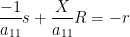
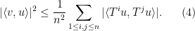
I recently learned about a curious operation on square matrices known as sweeping, which is used in numerical linear algebra (particularly in applications to statistics), as a useful and more robust variant of the usual Gaussian elimination operations seen in undergraduate linear algebra courses. Given an 


![{\hbox{Sweep}_k[A] = (\hat a_{ij})_{1 \leq i,j \leq n}}](https://s0.wp.com/latex.php?latex=%7B%5Chbox%7BSweep%7D_k%5BA%5D+%3D+%28%5Chat+a_%7Bij%7D%29_%7B1+%5Cleq+i%2Cj+%5Cleq+n%7D%7D&bg=ffffff&fg=000000&s=0&c=20201002)


for all 


for some 


![\displaystyle \hbox{Sweep}_1[A] = \begin{pmatrix} -1/a_{11} & X / a_{11} \\ Y/a_{11} & B - a_{11}^{-1} YX \end{pmatrix}. \ \ \ \ \ (2)](https://s0.wp.com/latex.php?latex=%5Cdisplaystyle++%5Chbox%7BSweep%7D_1%5BA%5D+%3D+%5Cbegin%7Bpmatrix%7D+-1%2Fa_%7B11%7D+%26+X+%2F+a_%7B11%7D+%5C%5C+Y%2Fa_%7B11%7D+%26+B+-+a_%7B11%7D%5E%7B-1%7D+YX+%5Cend%7Bpmatrix%7D.+%5C+%5C+%5C+%5C+%5C+%282%29&bg=ffffff&fg=000000&s=0&c=20201002)
The inverse sweep operation ![{\hbox{Sweep}_k^{-1}[A] = (\check a_{ij})_{1 \leq i,j \leq n}}](https://s0.wp.com/latex.php?latex=%7B%5Chbox%7BSweep%7D_k%5E%7B-1%7D%5BA%5D+%3D+%28%5Ccheck+a_%7Bij%7D%29_%7B1+%5Cleq+i%2Cj+%5Cleq+n%7D%7D&bg=ffffff&fg=000000&s=0&c=20201002)


for all 
Remarkably, the sweep operators all commute with each other: 
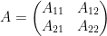
with 


![\displaystyle \hbox{Sweep}_1 \dots \hbox{Sweep}_k[A] = \begin{pmatrix} -A_{11}^{-1} & A_{11}^{-1} A_{12} \\ A_{21} A_{11}^{-1} & A_{22} - A_{21} A_{11}^{-1} A_{12} \end{pmatrix}.](https://s0.wp.com/latex.php?latex=%5Cdisplaystyle++%5Chbox%7BSweep%7D_1+%5Cdots+%5Chbox%7BSweep%7D_k%5BA%5D+%3D+%5Cbegin%7Bpmatrix%7D+-A_%7B11%7D%5E%7B-1%7D+%26+A_%7B11%7D%5E%7B-1%7D+A_%7B12%7D+%5C%5C+A_%7B21%7D+A_%7B11%7D%5E%7B-1%7D+%26+A_%7B22%7D+-+A_%7B21%7D+A_%7B11%7D%5E%7B-1%7D+A_%7B12%7D+%5Cend%7Bpmatrix%7D.&bg=ffffff&fg=000000&s=0&c=20201002)
Note the appearance of the Schur complement in the bottom right block. Thus, for instance, one can essentially invert a matrix
![\displaystyle \hbox{Sweep}_1 \dots \hbox{Sweep}_n[A] = -A^{-1}.](https://s0.wp.com/latex.php?latex=%5Cdisplaystyle++%5Chbox%7BSweep%7D_1+%5Cdots+%5Chbox%7BSweep%7D_n%5BA%5D+%3D+-A%5E%7B-1%7D.&bg=ffffff&fg=000000&s=0&c=20201002)
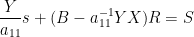
If a matrix has the form

for a 

![\displaystyle \hbox{Sweep}_1 \dots \hbox{Sweep}_{n-1}[A] = \begin{pmatrix} -B^{-1} & B^{-1} X \\ Y B^{-1} & a - Y B^{-1} X \end{pmatrix}](https://s0.wp.com/latex.php?latex=%5Cdisplaystyle++%5Chbox%7BSweep%7D_1+%5Cdots+%5Chbox%7BSweep%7D_%7Bn-1%7D%5BA%5D+%3D+%5Cbegin%7Bpmatrix%7D+-B%5E%7B-1%7D+%26+B%5E%7B-1%7D+X+%5C%5C+Y+B%5E%7B-1%7D+%26+a+-+Y+B%5E%7B-1%7D+X+%5Cend%7Bpmatrix%7D+&bg=ffffff&fg=000000&s=0&c=20201002)
and all the components of this matrix are usable for various numerical linear algebra applications in statistics (e.g. in least squares regression). Given that sweeps behave well with inverses, it is perhaps not surprising that sweeps also behave well under determinants: the determinant of ![{\hbox{Sweep}_k[A]}](https://s0.wp.com/latex.php?latex=%7B%5Chbox%7BSweep%7D_k%5BA%5D%7D&bg=ffffff&fg=000000&s=0&c=20201002)


It turns out that there is a simple geometric explanation for these seemingly magical properties of the sweep operation. Any ![{\hbox{Graph}[A] := \{ (X, AX): X \in {\bf R}^n \}}](https://s0.wp.com/latex.php?latex=%7B%5Chbox%7BGraph%7D%5BA%5D+%3A%3D+%5C%7B+%28X%2C+AX%29%3A+X+%5Cin+%7B%5Cbf+R%7D%5En+%5C%7D%7D&bg=ffffff&fg=000000&s=0&c=20201002)


We use 


![\displaystyle \hbox{Graph}[ \hbox{Sweep}_k[A] ] = \hbox{Rot}_k \hbox{Graph}[A]](https://s0.wp.com/latex.php?latex=%5Cdisplaystyle++%5Chbox%7BGraph%7D%5B+%5Chbox%7BSweep%7D_k%5BA%5D+%5D+%3D+%5Chbox%7BRot%7D_k+%5Chbox%7BGraph%7D%5BA%5D+&bg=ffffff&fg=000000&s=0&c=20201002)
for generic ![{\hbox{Graph}[A]}](https://s0.wp.com/latex.php?latex=%7B%5Chbox%7BGraph%7D%5BA%5D%7D&bg=ffffff&fg=000000&s=0&c=20201002)


The image of 


we see from (2) that ![{\hbox{Rot}_1 \hbox{Graph}[A]}](https://s0.wp.com/latex.php?latex=%7B%5Chbox%7BRot%7D_1+%5Chbox%7BGraph%7D%5BA%5D%7D&bg=ffffff&fg=000000&s=0&c=20201002)
![{\hbox{Sweep}_1[A]}](https://s0.wp.com/latex.php?latex=%7B%5Chbox%7BSweep%7D_1%5BA%5D%7D&bg=ffffff&fg=000000&s=0&c=20201002)


It is then an instructive exercise to use this geometric interpretation of the sweep operator to recover all the remarkable properties about these operations listed above. It is also useful to compare the geometric interpretation of sweeping as rotation of the graph to that of Gaussian elimination, which instead shears and reflects the graph by various elementary transformations (this is what is going on geometrically when one performs Gaussian elimination on an augmented matrix). Rotations are less distorting than shears, so one can see geometrically why sweeping can produce fewer numerical artefacts than Gaussian elimination.
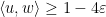
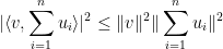
Given two unit vectors 


One can also define correlation for complex (Hermitian) inner product spaces by taking the real part 
While reading the (highly recommended) recent popular maths book “How not to be wrong“, by my friend and co-author Jordan Ellenberg, I came across the (important) point that correlation is not necessarily transitive: if 

in the Euclidean plane 


However, there are at least two situations in which some partial version of transitivity of correlation can be recovered. The first is in the “99%” regime in which the correlations are very close to 

(and similarly for 


Thus, for instance, if 


Remark 1 (Thanks to Andrew Granville for conversations leading to this observation.) The inequality (1) also holds for sub-unit vectors, i.e. vectors
. This comes by extending
if necessary. More concretely, one can apply (1) to the unit vectors
in
.

But even in the “

Thus, for instance, if 


A similar argument (multiplying each 

and this inequality is also true for complex inner product spaces. (Also, the
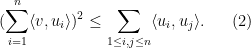
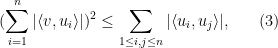
Geometrically, the picture is this: if 
A particularly common special case of the van der Corput inequality arises when 


(In fact, one can even remove the absolute values from the right-hand side, by using (2) instead of (4).) Thus, to show that
Here is a basic application of the van der Corput inequality:
Proposition 2 (Weyl equidistribution estimate) Let
be a polynomial with at least one non-constant coefficient irrational. Then one has
where
.

Note that this assertion implies the more general assertion

for any non-zero integer 


Proof: We induct on the degree 


In order to use the van der Corput inequality as stated above (i.e. in the formalism of inner product spaces) we will need a non-principal ultrafilter 
Strictly speaking, this inner product is only positive semi-definite rather than positive definite, but one can quotient out by the null vectors to obtain a positive-definite inner product. To establish the claim, it will suffice to show that

for every non-principal ultrafilter
Note that the space of bounded sequences (modulo null vectors) admits a shift

This shift becomes unitary once we quotient out by null vectors, and the constant sequence
for any 


for any 
A remarkable phenomenon in probability theory is that of universality – that many seemingly unrelated probability distributions, which ostensibly involve large numbers of unknown parameters, can end up converging to a universal law that may only depend on a small handful of parameters. One of the most famous examples of the universality phenomenon is the central limit theorem; another rich source of examples comes from random matrix theory, which is one of the areas of my own research.
Analogous universality phenomena also show up in empirical distributions – the distributions of a statistic
- (i) take values as positive numbers;
- (ii) range over many different orders of magnitude;
- (iiii) arise from a complicated combination of largely independent factors (with different samples of
- (iv) have not been artificially rounded, truncated, or otherwise constrained in size.
Examples here include the population of countries or cities, the frequency of occurrence of words in a language, the mass of astronomical objects, or the net worth of individuals or corporations. The laws are then as follows:
- Benford’s law: For
, the proportion of
. Thus, for instance,
- Zipf’s law: The
largest value of
for the first few
and some parameters
. In many cases,
is close to
- Pareto distribution: The proportion of
for some
. Again, in many cases
Benford’s law and Pareto distribution are stated here for base
To illustrate these laws, let us take as a data set the populations of 235 countries and regions of the world in 2007 (using the CIA world factbook); I have put the raw data here. This is a relatively small sample (cf. my previous post), but is already enough to discern these laws in action. For instance, here is how the data set tracks with Benford’s law (rounded to three significant figures):
| |
Countries | Number | Benford prediction |
| 1 | Angola, Anguilla, Aruba, Bangladesh, Belgium, Botswana, Brazil, Burkina Faso, Cambodia, Cameroon, Chad, Chile, China, Christmas Island, Cook Islands, Cuba, Czech Republic, Ecuador, Estonia, Gabon, (The) Gambia, Greece, Guam, Guatemala, Guinea-Bissau, India, Japan, Kazakhstan, Kiribati, Malawi, Mali, Mauritius, Mexico, (Federated States of) Micronesia, Nauru, Netherlands, Niger, Nigeria, Niue, Pakistan, Portugal, Russia, Rwanda, Saint Lucia, Saint Vincent and the Grenadines, Senegal, Serbia, Swaziland, Syria, Timor-Leste (East-Timor), Tokelau, Tonga, Trinidad and Tobago, Tunisia, Tuvalu, (U.S.) Virgin Islands, Wallis and Futuna, Zambia, Zimbabwe | 59 ( ) ) |
71 ( ) ) |
| 2 | Armenia, Australia, Barbados, British Virgin Islands, Cote d’Ivoire, French Polynesia, Ghana, Gibraltar, Indonesia, Iraq, Jamaica, (North) Korea, Kosovo, Kuwait, Latvia, Lesotho, Macedonia, Madagascar, Malaysia, Mayotte, Mongolia, Mozambique, Namibia, Nepal, Netherlands Antilles, New Caledonia Norfolk Island, Palau, Peru, Romania, Saint Martin, Samoa, San Marino, Sao Tome and Principe, Saudi Arabia, Slovenia, Sri Lanka, Svalbard, Taiwan, Turks and Caicos Islands, Uzbekistan, Vanuatu, Venezuela, Yemen | 44 ( ) ) |
41 ( ) ) |
| 3 | Afghanistan, Albania, Algeria, (The) Bahamas, Belize, Brunei, Canada, (Rep. of the) Congo, Falkland Islands (Islas Malvinas), Iceland, Kenya, Lebanon, Liberia, Liechtenstein, Lithuania, Maldives, Mauritania, Monaco, Morocco, Oman, (Occupied) Palestinian Territory, Panama, Poland, Puerto Rico, Saint Kitts and Nevis, Uganda, United States of America, Uruguay, Western Sahara | 29 ( ) ) |
29 ( ) ) |
| 4 | Argentina, Bosnia and Herzegovina, Burma (Myanmar), Cape Verde, Cayman Islands, Central African Republic, Colombia, Costa Rica, Croatia, Faroe Islands, Georgia, Ireland, (South) Korea, Luxembourg, Malta, Moldova, New Zealand, Norway, Pitcairn Islands, Singapore, South Africa, Spain, Sudan, Suriname, Tanzania, Ukraine, United Arab Emirates | 27 ( ) ) |
22 ( ) ) |
| 5 | (Macao SAR) China, Cocos Islands, Denmark, Djibouti, Eritrea, Finland, Greenland, Italy, Kyrgyzstan, Montserrat, Nicaragua, Papua New Guinea, Slovakia, Solomon Islands, Togo, Turkmenistan | 16 ( ) ) |
19 ( ) ) |
| 6 | American Samoa, Bermuda, Bhutan, (Dem. Rep. of the) Congo, Equatorial Guinea, France, Guernsey, Iran, Jordan, Laos, Libya, Marshall Islands, Montenegro, Paraguay, Sierra Leone, Thailand, United Kingdom | 17 ( ) ) |
16 ( ) ) |
| 7 | Bahrain, Bulgaria, (Hong Kong SAR) China, Comoros, Cyprus, Dominica, El Salvador, Guyana, Honduras, Israel, (Isle of) Man, Saint Barthelemy, Saint Helena, Saint Pierre and Miquelon, Switzerland, Tajikistan, Turkey | 17 () |
14 ( ) ) |
| 8 | Andorra, Antigua and Barbuda, Austria, Azerbaijan, Benin, Burundi, Egypt, Ethiopia, Germany, Haiti, Holy See (Vatican City), Northern Mariana Islands, Qatar, Seychelles, Vietnam | 15 ( ) ) |
12 ( ) ) |
| 9 | Belarus, Bolivia, Dominican Republic, Fiji, Grenada, Guinea, Hungary, Jersey, Philippines, Somalia, Sweden | 11 ( ) ) |
11 ( ) ) |
Here is how the same data tracks Zipf’s law for the first twenty values of 

| |
Country | Population | Zipf prediction | Deviation from prediction |
| 1 | China | 1,330,000,000 | 1,280,000,000 |  |
| 2 | India | 1,150,000,000 | 626,000,000 |  |
| 3 | USA | 304,000,000 | 412,000,000 |  |
| 4 | Indonesia | 238,000,000 | 307,000,000 |  |
| 5 | Brazil | 196,000,000 | 244,000,000 |  |
| 6 | Pakistan | 173,000,000 | 202,000,000 |  |
| 7 | Bangladesh | 154,000,000 | 172,000,000 |  |
| 8 | Nigeria | 146,000,000 | 150,000,000 |  |
| 9 | Russia | 141,000,000 | 133,000,000 |  |
| 10 | Japan | 128,000,000 | 120,000,000 |  |
| 11 | Mexico | 110,000,000 | 108,000,000 |  |
| 12 | Philippines | 96,100,000 | 98,900,000 |  |
| 13 | Vietnam | 86,100,000 | 91,100,000 |  |
| 14 | Ethiopia | 82,600,000 | 84,400,000 |  |
| 15 | Germany | 82,400,000 | 78,600,000 |  |
| 16 | Egypt | 81,700,000 | 73,500,000 |  |
| 17 | Turkey | 71,900,000 | 69,100,000 | |
| 18 | Congo | 66,500,000 | 65,100,000 |  |
| 19 | Iran | 65,900,000 | 61,600,000 |  |
| 20 | Thailand | 65,500,000 | 58,400,000 |  |
As one sees, Zipf’s law is not particularly precise at the extreme edge of the statistics (when
This data set has too few scales in base 


| |
Countries with  binary digit populations binary digit populations |
Number | Pareto prediction |
| 31 | China, India | 2 | 1 |
| 30 | ” | 2 | 2 |
| 29 | “, United States of America | 3 | 5 |
| 28 | “, Indonesia, Brazil, Pakistan, Bangladesh, Nigeria, Russia | 9 | 8 |
| 27 | “, Japan, Mexico, Philippines, Vietnam, Ethiopia, Germany, Egypt, Turkey | 17 | 15 |
| 26 | “, (Dem. Rep. of the) Congo, Iran, Thailand, France, United Kingdom, Italy, South Africa, (South) Korea, Burma (Myanmar), Ukraine, Colombia, Spain, Argentina, Sudan, Tanzania, Poland, Kenya, Morocco, Algeria | 36 | 27 |
| 25 | “, Canada, Afghanistan, Uganda, Nepal, Peru, Iraq, Saudi Arabia, Uzbekistan, Venezuela, Malaysia, (North) Korea, Ghana, Yemen, Taiwan, Romania, Mozambique, Sri Lanka, Australia, Cote d’Ivoire, Madagascar, Syria, Cameroon | 58 | 49 |
| 24 | “, Netherlands, Chile, Kazakhstan, Burkina Faso, Cambodia, Malawi, Ecuador, Niger, Guatemala, Senegal, Angola, Mali, Zambia, Cuba, Zimbabwe, Greece, Portugal, Belgium, Tunisia, Czech Republic, Rwanda, Serbia, Chad, Hungary, Guinea, Belarus, Somalia, Dominican Republic, Bolivia, Sweden, Haiti, Burundi, Benin | 91 | 88 |
| 23 | “, Austria, Azerbaijan, Honduras, Switzerland, Bulgaria, Tajikistan, Israel, El Salvador, (Hong Kong SAR) China, Paraguay, Laos, Sierra Leone, Jordan, Libya, Papua New Guinea, Togo, Nicaragua, Eritrea, Denmark, Slovakia, Kyrgyzstan, Finland, Turkmenistan, Norway, Georgia, United Arab Emirates, Singapore, Bosnia and Herzegovina, Croatia, Central African Republic, Moldova, Costa Rica | 123 | 159 |
Thus, with each new scale, the number of countries introduced increases by a factor of a little less than 
These laws are not merely interesting statistical curiosities; for instance, Benford’s law is often used to help detect fraudulent statistics (such as those arising from accounting fraud), as many such statistics are invented by choosing digits at random, and will therefore deviate significantly from Benford’s law. (This is nicely discussed in Robert Matthews’ New Scientist article “The power of one“; this article can also be found on the web at a number of other places.) In a somewhat analogous spirit, Zipf’s law and the Pareto distribution can be used to mathematically test various models of real-world systems (e.g. formation of astronomical objects, accumulation of wealth, population growth of countries, etc.), without necessarily having to fit all the parameters of that model with the actual data.
Being empirically observed phenomena rather than abstract mathematical facts, Benford’s law, Zipf’s law, and the Pareto distribution cannot be “proved” the same way a mathematical theorem can be proved. However, one can still support these laws mathematically in a number of ways, for instance showing how these laws are compatible with each other, and with other plausible hypotheses on the source of the data. In this post I would like to describe a number of ways (both technical and non-technical) in which one can do this; these arguments do not fully explain these laws (in particular, the empirical fact that the exponent
The U.S. presidential election is now only a few weeks away. The politics of this election are of course interesting and important, but I do not want to discuss these topics here (there is not exactly a shortage of other venues for such a discussion), and would request that readers refrain from doing so in the comments to this post. However, I thought it would be apropos to talk about some of the basic mathematics underlying electoral polling, and specifically to explain the fact, which can be highly unintuitive to those not well versed in statistics, that polls can be accurate even when sampling only a tiny fraction of the entire population.
Take for instance a nationwide poll of U.S. voters on which presidential candidate they intend to vote for. A typical poll will ask a number 


I’ll give a rigorous proof of a weaker version of the above statement (giving a margin of error of about 7%, rather than 3%) in an appendix at the end of this post. But the main point of my post here is a little different, namely to address the common misconception that the accuracy of a poll is a function of the relative sample size rather than the absolute sample size, which would suggest that a poll involving only 0.0005% of the population could not possibly have a margin of error as low as 3%. I also want to point out some limitations of the mathematical analysis; depending on the methodology and the context, some polls involving 1000 respondents may have a much higher margin of error than the idealised rate of 3%.

Recent Comments