
You are currently browsing the category archive for the ‘polymath’ category.
After some discussion with the applied math research groups here at UCLA (in particular the groups led by Andrea Bertozzi and Deanna Needell), one of the members of these groups, Chris Strohmeier, has produced a proposal for a Polymath project to crowdsource in a single repository (a) a collection of public data sets relating to the COVID-19 pandemic, (b) requests for such data sets, (c) requests for data cleaning of such sets, and (d) submissions of cleaned data sets. (The proposal can be viewed as a PDF, and is also available on Overleaf). As mentioned in the proposal, this database would be slightly different in focus than existing data sets such as the COVID-19 data sets hosted on Kaggle, with a focus on producing high quality cleaned data sets. (Another relevant data set that I am aware of is the SafeGraph aggregated foot traffic data, although this data set, while open, is not quite public as it requires a non-commercial agreement to execute. Feel free to mention further relevant data sets in the comments.)
This seems like a very interesting and timely proposal to me and I would like to open it up for discussion, for instance by proposing some seed requests for data and data cleaning and to discuss possible platforms that such a repository could be built on. In the spirit of “building the plane while flying it”, one could begin by creating a basic github repository as a prototype and use the comments in this blog post to handle requests, and then migrate to a more high quality platform once it becomes clear what direction this project might move in. (For instance one might eventually move beyond data cleaning to more sophisticated types of data analysis.)
UPDATE, Mar 25: a prototype page for such a clearinghouse is now up at this wiki page.
UPDATE, Mar 27: the data cleaning aspect of this project largely duplicates the existing efforts at the United against COVID-19 project, so we are redirecting requests of this type to that project (and specifically to their data discourse page). The polymath proposal will now refocus on crowdsourcing a list of public data sets relating to the COVID-19 pandemic.
The Polymath15 paper “Effective approximation of heat flow evolution of the Riemann 

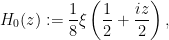
where
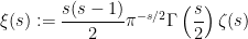
has a Fourier representation
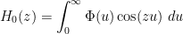
where 
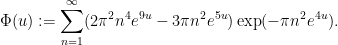
The Riemann hypothesis is equivalent to the claim that all the zeroes of 

of 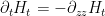


with the lower bound due to Rodgers and myself, and the upper bound due to Ki, Kim, and Lee. One of the main results of the paper is to improve the upper bound to

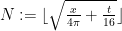
At a purely numerical level this gets “closer” to proving the Riemann hypothesis, but the methods of proof take as input a finite numerical verification of the Riemann hypothesis up to some given height 


We now discuss the methods of proof. An existing result of de Bruijn shows that if all the zeroes of 


whenever 

For large 


for 


for 
To enforce this barrier, and to verify (2) for large 
where 


where 


The most difficult computational task is the verification of the barrier (3), particularly when 


This post can serve as the (presumably final) thread for the Polymath15 project (continuing this post), to handle any remaining discussion topics for that project.
This is the eleventh research thread of the Polymath15 project to upper bound the de Bruijn-Newman constant 
There are currently two strands of activity. One is writing up the paper describing the combination of theoretical and numerical results needed to obtain the new bound 
- giving a more detailed description and illustration of the two major numerical verifications, namely the barrier verification that establishes a zero-free region for
for
, and the Dirichlet series bound that establishes a zero-free region for
; and
- giving more detail on the conditional results assuming more numerical verification of RH.
Meanwhile, several of us have been exploring the behaviour of the zeroes of 


(An example of the agreement between the zeroes and these curves may be found here.) We now have a (heuristic) theoretical explanation for this; we should have an approximation
in this region (where 


However, we only have a partial explanation at present of the interesting behaviour of the real zeroes at negative t, for instance the surviving zeroes at extremely negative values of 


The remaining zeroes exhibit a pattern in 

A plot of the zeroes in these coordinates (somewhat truncated due to the numerical range) may be found here.
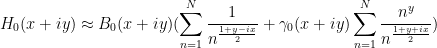
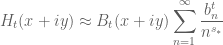
We do not yet have a total explanation of the phenomena seen in this picture. It appears that we have an approximation
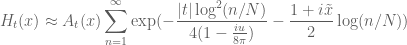
where 
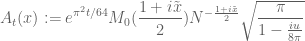
and

The derivation of this formula may be found in this wiki page. However our initial attempts to simplify the above approximation further have proven to be somewhat inaccurate numerically (in particular giving an incorrect prediction for the location of zeroes, as seen in this picture). We are in the process of using numerics to try to resolve the discrepancies (see this page for some code and discussion).
This is the tenth “research” thread of the Polymath15 project to upper bound the de Bruijn-Newman constant
Most of the progress since the last thread has been on the numerical side, in which the various techniques to numerically establish zero-free regions to the equation 


As progress seems to have stabilised, it may be time to transition to the writing phase of the Polymath15 project. (There are still some interesting research questions to pursue, such as numerically investigating the zeroes of
Below the fold is the detailed progress report on the numerics by Rudolph Dwars and Kalpesh Muchhal.
This is the ninth “research” thread of the Polymath15 project to upper bound the de Bruijn-Newman constant
We have now tentatively improved the upper bound of the de Bruijn-Newman constant to 


The main remaining bottleneck is that of computing the Euler mollifier bounds that keep 
Participants are also welcome to add any further summaries of the situation in the comments below.
Just a quick announcement that Dustin Mixon and Aubrey de Grey have just launched the Polymath16 project over at Dustin’s blog. The main goal of this project is to simplify the recent proof by Aubrey de Grey that the chromatic number of the unit distance graph of the plane is at least 5, thus making progress on the Hadwiger-Nelson problem. The current proof is computer assisted (in particular it requires one to control the possible 4-colorings of a certain graph with over a thousand vertices), but one of the aims of the project is to reduce the amount of computer assistance needed to verify the proof; already a number of such reductions have been found. See also this blog post where the polymath project was proposed, as well as the wiki page for the project. Non-technical discussion of the project will continue at the proposal blog post.
This is the seventh “research” thread of the Polymath15 project to upper bound the de Bruijn-Newman constant
The most recent news is that we appear to have completed the verification that 


One obvious thing to do now is to experiment with lowering the parameters 


Another, rather different approach, is to study the evolution of statistics such as 

Participants are also welcome to add any further summaries of the situation in the comments below.
This is the sixth “research” thread of the Polymath15 project to upper bound the de Bruijn-Newman constant
The last two threads have been focused primarily on the test problem of showing that 


has been proven for certain explicit expressions 

then 
We have explicit upper bounds on 


Meanwhile, the quantity 

for certain explicit coefficients 

we can obtain a lower bound of 


In the range 


This leaves the final range 


Beyond this, we need to figure out how to show that 

The full argument also needs to be streamlined and organised; right now it sprawls over many wiki pages and github code files. (A very preliminary writeup attempt has begun here). We should also see if there is much hope of extending the methods to push much beyond the bound of
Participants are also welcome to add any further summaries of the situation in the comments below.
This is the fifth “research” thread of the Polymath15 project to upper bound the de Bruijn-Newman constant
We have almost finished off the test problem of showing that

where the expressions 


The ratio 


As before, any other mathematical discussion related to the project is also welcome here, for instance any summaries of previous discussion that was not covered in this post.
This is the fourth “research” thread of the Polymath15 project to upper bound the de Bruijn-Newman constant
We are getting closer to finishing off the following test problem: can one show that 

for some explicit (but somewhat messy) error terms 

It is convenient to normalise everything by an explicit non-zero factor 


In addition to this main direction of inquiry, there have been additional discussions on the dynamics of zeroes, and some numerical investigations of the behaviour Lehmer pairs under heat flow. Contributors are welcome to summarise any findings from these discussions from previous threads (or on any other related topic, e.g. improvements in the code) in the comments below.

Recent Comments