Tag Archive

You are currently browsing the tag archive for the ‘Navier-Stokes equations’ tag.

Quantitative bounds for critically bounded solutions to the Navier-Stokes equations

15 August, 2019 in math.AP, paper | Tags: hard analysis, Navier-Stokes equations | by Terence Tao | 52 comments

I’ve just uploaded to the arXiv my paper “Quantitative bounds for critically bounded solutions to the Navier-Stokes equations“, submitted to the proceedings of the Linde Hall Inaugural Math Symposium. (I unfortunately had to cancel my physical attendance at this symposium for personal reasons, but was still able to contribute to the proceedings.) In recent years I have been interested in working towards establishing the existence of classical solutions for the Navier-Stokes equations

$\displaystyle \partial_t u + (u \cdot \nabla) u = \Delta u - \nabla p$

$\displaystyle \nabla \cdot u = 0$

that blow up in finite time, but this time for a change I took a look at the other side of the theory, namely the conditional regularity results for this equation. There are several such results that assert that if a certain norm of the solution stays bounded (or grows at a controlled rate), then the solution stays regular; taken in the contrapositive, they assert that if a solution blows up at a certain finite time ${T_*}$ , then certain norms of the solution must also go to infinity. Here are some examples (not an exhaustive list) of such blowup criteria:

(Leray blowup criterion, 1934) If ${u}$ blows up at a finite time ${T_*}$ , and ${3 < p \leq \infty}$ , then ${\liminf_{t \rightarrow T_*} (T_* - t)^{\frac{1}{2}-\frac{3}{2p}} \| u(t) \|_{L^p_x({\bf R}^3)} \geq c}$ for an absolute constant ${c>0}$ .
(Prodi–Serrin–Ladyzhenskaya blowup criterion, 1959-1967) If ${u}$ blows up at a finite time ${T_*}$ , and ${3 < p \leq \infty}$ , then ${\| u \|_{L^q_t L^p_x([0,T_*) \times {\bf R}^3)} =+\infty}$ , where ${\frac{1}{q} := \frac{1}{2} - \frac{3}{2p}}$ .
(Beale-Kato-Majda blowup criterion, 1984) If ${u}$ blows up at a finite time ${T_*}$ , then ${\| \omega \|_{L^1_t L^\infty_x([0,T_*) \times {\bf R}^3)} = +\infty}$ , where ${\omega := \nabla \times u}$ is the vorticity.
(Kato blowup criterion, 1984) If ${u}$ blows up at a finite time ${T_*}$ , then ${\liminf_{t \rightarrow T_*} \|u(t) \|_{L^3_x({\bf R}^3)} \geq c}$ for some absolute constant ${c>0}$ .
(Escauriaza-Seregin-Sverak blowup criterion, 2003) If ${u}$ blows up at a finite time ${T_*}$ , then ${\limsup_{t \rightarrow T_*} \|u(t) \|_{L^3_x({\bf R}^3)} = +\infty}$ .
(Seregin blowup criterion, 2012) If ${u}$ blows up at a finite time ${T_*}$ , then ${\lim_{t \rightarrow T_*} \|u(t) \|_{L^3_x({\bf R}^3)} = +\infty}$ .
(Phuc blowup criterion, 2015) If ${u}$ blows up at a finite time ${T_*}$ , then ${\limsup_{t \rightarrow T_*} \|u(t) \|_{L^{3,q}_x({\bf R}^3)} = +\infty}$ for any ${q < \infty}$ .
(Gallagher-Koch-Planchon blowup criterion, 2016) If ${u}$ blows up at a finite time ${T_*}$ , then ${\limsup_{t \rightarrow T_*} \|u(t) \|_{\dot B_{p,q}^{-1+3/p}({\bf R}^3)} = +\infty}$ for any ${3 < p, q < \infty}$ .
(Albritton blowup criterion, 2016) If ${u}$ blows up at a finite time ${T_*}$ , then ${\lim_{t \rightarrow T_*} \|u(t) \|_{\dot B_{p,q}^{-1+3/p}({\bf R}^3)} = +\infty}$ for any ${3 < p, q < \infty}$ .

My current paper is most closely related to the Escauriaza-Seregin-Sverak blowup criterion, which was the first to show a critical (i.e., scale-invariant, or dimensionless) spatial norm, namely ${L^3_x({\bf R}^3)}$ , had to become large. This result now has many proofs; for instance, many of the subsequent blowup criterion results imply the Escauriaza-Seregin-Sverak one as a special case, and there are also additional proofs by Gallagher-Koch-Planchon (building on ideas of Kenig-Koch), and by Dong-Du. However, all of these proofs rely on some form of a compactness argument: given a finite time blowup, one extracts some suitable family of rescaled solutions that converges in some weak sense to a limiting solution that has some additional good properties (such as almost periodicity modulo symmetries), which one can then rule out using additional qualitative tools, such as unique continuation and backwards uniqueness theorems for parabolic heat equations. In particular, all known proofs use some version of the backwards uniqueness theorem of Escauriaza, Seregin, and Sverak. Because of this reliance on compactness, the existing proofs of the Escauriaza-Seregin-Sverak blowup criterion are qualitative, in that they do not provide any quantitative information on how fast the ${\|u(t)\|_{L^3_x({\bf R}^3)}}$ norm will go to infinity (along a subsequence of times).

On the other hand, it is a general principle that qualitative arguments established using compactness methods ought to have quantitative analogues that replace the use of compactness by more complicated substitutes that give effective bounds; see for instance these previous blog posts for more discussion. I therefore was interested in trying to obtain a quantitative version of this blowup criterion that gave reasonably good effective bounds (in particular, my objective was to avoid truly enormous bounds such as tower-exponential or Ackermann function bounds, which often arise if one “naively” tries to make a compactness argument effective). In particular, I obtained the following triple-exponential quantitative regularity bounds:

Theorem 1 If ${u}$ is a classical solution to Navier-Stokes on ${[0,T) \times {\bf R}^3}$ with

$\displaystyle \| u \|_{L^\infty_t L^3_x([0,T) \times {\bf R}^3)} \leq A \ \ \ \ \ (1)$

for some ${A \geq 2}$ , then

$\displaystyle | \nabla^j u(t,x)| \leq \exp\exp\exp(A^{O(1)}) t^{-\frac{j+1}{2}}$

and

$\displaystyle | \nabla^j \omega(t,x)| \leq \exp\exp\exp(A^{O(1)}) t^{-\frac{j+2}{2}}$

for ${(t,x) \in [0,T) \times {\bf R}^3}$ and ${j=0,1}$ .

As a corollary, one can now improve the Escauriaza-Seregin-Sverak blowup criterion to

$\displaystyle \limsup_{t \rightarrow T_*} \frac{\|u(t) \|_{L^3_x({\bf R}^3)}}{(\log\log\log \frac{1}{T_*-t})^c} = +\infty$

for some absolute constant ${c>0}$ , which to my knowledge is the first (very slightly) supercritical blowup criterion for Navier-Stokes in the literature.

The proof uses many of the same quantitative inputs as previous arguments, most notably the Carleman inequalities used to establish unique continuation and backwards uniqueness theorems for backwards heat equations, but also some additional techniques that make the quantitative bounds more efficient. The proof focuses initially on points of concentration of the solution, which we define as points ${(t_0,x_0)}$ where there is a frequency ${N_0}$ for which one has the bound

$\displaystyle |N_0^{-1} P_{N_0} u(t_0,x_0)| \geq A^{-C_0} \ \ \ \ \ (2)$

for a large absolute constant ${C_0}$ , where ${P_{N_0}}$ is a Littlewood-Paley projection to frequencies ${\sim N_0}$ . (This can be compared with the upper bound of ${O(A)}$ for the quantity on the left-hand side that follows from (1).) The factor of ${N_0^{-1}}$ normalises the left-hand side of (2) to be dimensionless (i.e., critical). The main task is to show that the dimensionless quantity ${t_0 N_0^2}$ cannot get too large; in particular, we end up establishing a bound of the form

$\displaystyle t_0 N_0^2 \lesssim \exp\exp\exp A^{O(C_0^6)}$

from which the above theorem ends up following from a routine adaptation of the local well-posedness and regularity theory for Navier-Stokes.

The strategy is to show that any concentration such as (2) when ${t_0 N_0^2}$ is large must force a significant component of the ${L^3_x}$ norm of ${u(t_0)}$ to also show up at many other locations than ${x_0}$ , which eventually contradicts (1) if one can produce enough such regions of non-trivial ${L^3_x}$ norm. (This can be viewed as a quantitative variant of the “rigidity” theorems in some of the previous proofs of the Escauriaza-Seregin-Sverak theorem that rule out solutions that exhibit too much “compactness” or “almost periodicity” in the ${L^3_x}$ topology.) The chain of causality that leads from a concentration (2) at ${(t_0,x_0)}$ to significant ${L^3_x}$ norm at other regions of the time slice ${t_0 \times {\bf R}^3}$ is somewhat involved (though simpler than the much more convoluted schemes I initially envisaged for this argument):

Firstly, by using Duhamel’s formula, one can show that a concentration (2) can only occur (with ${t_0 N_0^2}$ large) if there was also a preceding concentration
$\displaystyle |N_1^{-1} P_{N_1} u(t_1,x_1)| \geq A^{-C_0} \ \ \ \ \ (3)$

at some slightly previous point ${(t_1,x_1)}$ in spacetime, with ${N_1}$ also close to ${N_0}$ (more precisely, we have ${t_1 = t_0 - A^{-O(C_0^3)} N_0^{-2}}$ , ${N_1 = A^{O(C_0^2)} N_0}$ , and ${x_1 = x_0 + O( A^{O(C_0^4)} N_0^{-1})}$ ). This can be viewed as a sort of contrapositive of a “local regularity theorem”, such as the ones established by Caffarelli, Kohn, and Nirenberg. A key point here is that the lower bound ${A^{-C_0}}$ in the conclusion (3) is precisely the same as the lower bound in (2), so that this backwards propagation of concentration can be iterated.
Iterating the previous step, one can find a sequence of concentration points
$\displaystyle |N_n^{-1} P_{N_n} u(t_n,x_n)| \geq A^{-C_0} \ \ \ \ \ (4)$

with the ${(t_n,x_n)}$ propagating backwards in time; by using estimates ultimately resulting from the dissipative term in the energy identity, one can extract such a sequence in which the ${t_0-t_n}$ increase geometrically with time, the ${N_n}$ are comparable (up to polynomial factors in ${A}$ ) to the natural frequency scale ${(t_0-t_n)^{-1/2}}$ , and one has ${x_n = x_0 + O( |t_0-t_n|^{1/2} )}$ . 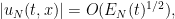Using the “epochs of regularity” theory that ultimately dates back to Leray, and tweaking the ${t_n}$ slightly, one can also place the times ${t_n}$ in intervals ${I_n}$ (of length comparable to a small multiple of ${|t_0-t_n|}$ ) in which the solution is quite regular (in particular, ${u, \nabla u, \omega, \nabla \omega}$ enjoy good ${L^\infty_t L^\infty_x}$ bounds on ${I_n \times {\bf R}^3}$ ).
The concentration (4) can be used to establish a lower bound for the ${L^2_t L^2_x}$ norm of the vorticity ${\omega}$ near ${(t_n,x_n)}$ . As is well known, the vorticity obeys the vorticity equation
$\displaystyle \partial_t \omega = \Delta \omega - (u \cdot \nabla) \omega + (\omega \cdot \nabla) u.$

In the epoch of regularity ${I_n \times {\bf R}^3}$ , the coefficients ${u, \nabla u}$ of this equation obey good ${L^\infty_x}$ bounds, allowing the machinery of Carleman estimates to come into play. Using a Carleman estimate that is used to establish unique continuation results for backwards heat equations, one can propagate this lower bound to also give lower ${L^2}$ bounds on the vorticity (and its first derivative) in annuli of the form ${\{ (t,x) \in I_n \times {\bf R}^3: R \leq |x-x_n| \leq R' \}}$ for various radii ${R,R'}$ , although the lower bounds decay at a gaussian rate with ${R}$ .
Meanwhile, using an energy pigeonholing argument of Bourgain (which, in this Navier-Stokes context, is actually an enstrophy pigeonholing argument), one can locate some annuli ${\{ x \in {\bf R}^3: R \leq |x-x_n| \leq R'\}}$ where (a slightly normalised form of) the entrosphy is small at time ${t=t_n}$ ; using a version of the localised enstrophy estimates from a previous paper of mine, one can then propagate this sort of control forward in time, obtaining an “annulus of regularity” of the form ${\{ (t,x) \in [t_n,t_0] \times {\bf R}^3: R_n \leq |x-x_n| \leq R'_n\}}$ in which one has good estimates; in particular, one has ${L^\infty_x}$ type bounds on ${u, \nabla u, \omega, \nabla \omega}$ in this cylindrical annulus.
By intersecting the previous epoch of regularity ${I_n \times {\bf R}^3}$ with the above annulus of regularity, we have some lower bounds on the ${L^2}$ norm of the vorticity (and its first derivative) in the annulus of regularity. Using a Carleman estimate first introduced by Escauriaza, Seregin, and Sverak, as well as a second application of the Carleman estimate used previously, one can then propagate this lower bound back up to time ${t=t_0}$ , establishing a lower bound for the vorticity on the spatial annulus ${\{ (t_0,x): R_n \leq |x-x_n| \leq R'_n \}}$ . By some basic Littlewood-Paley theory one can parlay this lower bound to a lower bound on the ${L^3}$ norm of the velocity ${u}$ ; crucially, this lower bound is uniform in ${n}$ .
If ${t_0 N_0^2}$ is very large (triple exponential in ${A}$ !), one can then find enough scales ${n}$ with disjoint ${\{ (t_0,x): R_n \leq |x-x_n| \leq R'_n \}}$ annuli that the total lower bound on the ${L^3_x}$ norm of ${u(t_0)}$ provided by the above arguments is inconsistent with (1), thus establishing the claim.

The chain of causality is summarised in the following image:

scheme

It seems natural to conjecture that similar triply logarithmic improvements can be made to several of the other blowup criteria listed above, but I have not attempted to pursue this question. It seems difficult to improve the triple logarithmic factor using only the techniques here; the Bourgain pigeonholing argument inevitably costs one exponential, the Carleman inequalities cost a second, and the stacking of scales at the end to contradict the ${L^3}$ upper bound costs the third.

Searching for singularities in the Navier–Stokes equations

31 May, 2019 in expository, math.AP, math.MP, paper | Tags: Navier-Stokes equations | by Terence Tao | 30 comments

I was recently asked to contribute a short comment to Nature Reviews Physics, as part of a series of articles on fluid dynamics on the occasion of the 200th anniversary (this August) of the birthday of George Stokes. My contribution is now online as “Searching for singularities in the Navier–Stokes equations“, where I discuss the global regularity problem for Navier-Stokes and my thoughts on how one could try to construct a solution that blows up in finite time via an approximately discretely self-similar “fluid computer”. (The rest of the series does not currently seem to be available online, but I expect they will become so shortly.)

254A, Notes 2: Weak solutions of the Navier-Stokes equations

2 October, 2018 in 254A - Incompressible fluid equations, math.AP, math.CA | Tags: compactness, distributions, Navier-Stokes equations, weak solutions | by Terence Tao | 48 comments

In the previous set of notes we developed a theory of “strong” solutions to the Navier-Stokes equations. This theory, based around viewing the Navier-Stokes equations as a perturbation of the linear heat equation, has many attractive features: solutions exist locally, are unique, depend continuously on the initial data, have a high degree of regularity, can be continued in time as long as a sufficiently high regularity norm is under control, and tend to enjoy the same sort of conservation laws that classical solutions do. However, it is a major open problem as to whether these solutions can be extended to be (forward) global in time, because the norms that we know how to control globally in time do not have high enough regularity to be useful for continuing the solution. Also, the theory becomes degenerate in the inviscid limit ${\nu \rightarrow 0}$ .

However, it is possible to construct “weak” solutions which lack many of the desirable features of strong solutions (notably, uniqueness, propagation of regularity, and conservation laws) but can often be constructed globally in time even when one us unable to do so for strong solutions. Broadly speaking, one usually constructs weak solutions by some sort of “compactness method”, which can generally be described as follows.

Construct a sequence of “approximate solutions” to the desired equation, for instance by developing a well-posedness theory for some “regularised” approximation to the original equation. (This theory often follows similar lines to those in the previous set of notes, for instance using such tools as the contraction mapping theorem to construct the approximate solutions.)
Establish some uniform bounds (over appropriate time intervals) on these approximate solutions, even in the limit as an approximation parameter is sent to zero. (Uniformity is key; non-uniform bounds are often easy to obtain if one puts enough “mollification”, “hyper-dissipation”, or “discretisation” in the approximating equation.)
Use some sort of “weak compactness” (e.g., the Banach-Alaoglu theorem, the Arzela-Ascoli theorem, or the Rellich compactness theorem) to extract a subsequence of approximate solutions that converge (in a topology weaker than that associated to the available uniform bounds) to a limit. (Note that there is no reason a priori to expect such limit points to be unique, or to have any regularity properties beyond that implied by the available uniform bounds..)
Show that this limit solves the original equation in a suitable weak sense.

The quality of these weak solutions is very much determined by the type of uniform bounds one can obtain on the approximate solution; the stronger these bounds are, the more properties one can obtain on these weak solutions. For instance, if the approximate solutions enjoy an energy identity leading to uniform energy bounds, then (by using tools such as Fatou’s lemma) one tends to obtain energy inequalities for the resulting weak solution; but if one somehow is able to obtain uniform bounds in a higher regularity norm than the energy then one can often recover the full energy identity. If the uniform bounds are at the regularity level needed to obtain well-posedness, then one generally expects to upgrade the weak solution to a strong solution. (This phenomenon is often formalised through weak-strong uniqueness theorems, which we will discuss later in these notes.) Thus we see that as far as attacking global regularity is concerned, both the theory of strong solutions and the theory of weak solutions encounter essentially the same obstacle, namely the inability to obtain uniform bounds on (exact or approximate) solutions at high regularities (and at arbitrary times).

For simplicity, we will focus our discussion in this notes on finite energy weak solutions on ${{\bf R}^d}$ . There is a completely analogous theory for periodic weak solutions on ${{\bf R}^d}$ (or equivalently, weak solutions on the torus ${({\bf R}^d/{\bf Z}^d)}$ which we will leave to the interested reader.

In recent years, a completely different way to construct weak solutions to the Navier-Stokes or Euler equations has been developed that are not based on the above compactness methods, but instead based on techniques of convex integration. These will be discussed in a later set of notes.

Read the rest of this entry »

254A, Notes 0: Physical derivation of the incompressible Euler and Navier-Stokes equations

3 September, 2018 in 254A - Incompressible fluid equations, math.AP, math.DS, math.MP | Tags: conservation laws, incompressible Euler equations, many-particle systems, Navier-Stokes equations, Newton's laws of motion | by Terence Tao | 41 comments

This coming fall quarter, I am teaching a class on topics in the mathematical theory of incompressible fluid equations, focusing particularly on the incompressible Euler and Navier-Stokes equations. These two equations are by no means the only equations used to model fluids, but I will focus on these two equations in this course to narrow the focus down to something manageable. I have not fully decided on the choice of topics to cover in this course, but I would probably begin with some core topics such as local well-posedness theory and blowup criteria, conservation laws, and construction of weak solutions, then move on to some topics such as boundary layers and the Prandtl equations, the Euler-Poincare-Arnold interpretation of the Euler equations as an infinite dimensional geodesic flow, and some discussion of the Onsager conjecture. I will probably also continue to more advanced and recent topics in the winter quarter.

In this initial set of notes, we begin by reviewing the physical derivation of the Euler and Navier-Stokes equations from the first principles of Newtonian mechanics, and specifically from Newton’s famous three laws of motion. Strictly speaking, this derivation is not needed for the mathematical analysis of these equations, which can be viewed if one wishes as an arbitrarily chosen system of partial differential equations without any physical motivation; however, I feel that the derivation sheds some insight and intuition on these equations, and is also worth knowing on purely intellectual grounds regardless of its mathematical consequences. I also find it instructive to actually see the journey from Newton’s law

$\displaystyle F = ma$

to the seemingly rather different-looking law

$\displaystyle \partial_t u + (u \cdot \nabla) u = -\nabla p + \nu \Delta u$

$\displaystyle \nabla \cdot u = 0$

for incompressible Navier-Stokes (or, if one drops the viscosity term ${\nu \Delta u}$ , the Euler equations).

Our discussion in this set of notes is physical rather than mathematical, and so we will not be working at mathematical levels of rigour and precision. In particular we will be fairly casual about interchanging summations, limits, and integrals, we will manipulate approximate identities ${X \approx Y}$ as if they were exact identities (e.g., by differentiating both sides of the approximate identity), and we will not attempt to verify any regularity or convergence hypotheses in the expressions being manipulated. (The same holds for the exercises in this text, which also do not need to be justified at mathematical levels of rigour.) Of course, once we resume the mathematical portion of this course in subsequent notes, such issues will be an important focus of careful attention. This is a basic division of labour in mathematical modeling: non-rigorous heuristic reasoning is used to derive a mathematical model from physical (or other “real-life”) principles, but once a precise model is obtained, the analysis of that model should be completely rigorous if at all possible (even if this requires applying the model to regimes which do not correspond to the original physical motivation of that model). See the discussion by John Ball quoted at the end of these slides of Gero Friesecke for an expansion of these points.

Note: our treatment here will differ slightly from that presented in many fluid mechanics texts, in that it will emphasise first-principles derivations from many-particle systems, rather than relying on bulk laws of physics, such as the laws of thermodynamics, which we will not cover here. (However, the derivations from bulk laws tend to be more robust, in that they are not as reliant on assumptions about the particular interactions between particles. In particular, the physical hypotheses we assume in this post are probably quite a bit stronger than the minimal assumptions needed to justify the Euler or Navier-Stokes equations, which can hold even in situations in which one or more of the hypotheses assumed here break down.)

Read the rest of this entry »

Kolmogorov’s power law for turbulence

15 May, 2014 in expository, math.AP, math.MP | Tags: dimensional analysis, Kolmogorov power law, Navier-Stokes equations, turbulence | by Terence Tao | 25 comments

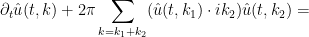
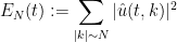
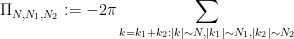
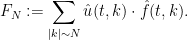
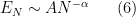
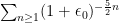
Many fluid equations are expected to exhibit turbulence in their solutions, in which a significant portion of their energy ends up in high frequency modes. A typical example arises from the three-dimensional periodic Navier-Stokes equations

$\displaystyle \partial_t u + u \cdot \nabla u = \nu \Delta u - \nabla p + f$

$\displaystyle \nabla \cdot u = 0$

where ${u: {\bf R} \times {\bf R}^3/{\bf Z}^3 \rightarrow {\bf R}^3}$ is the velocity field, ${f: {\bf R} \times {\bf R}^3/{\bf Z}^3 \rightarrow {\bf R}^3}$ is a forcing term, ${p: {\bf R} \times {\bf R}^3/{\bf Z}^3 \rightarrow {\bf R}}$ is a pressure field, and ${\nu > 0}$ is the viscosity. To study the dynamics of energy for this system, we first pass to the Fourier transform

$\displaystyle \hat u(t,k) := \int_{{\bf R}^3/{\bf Z}^3} u(t,x) e^{-2\pi i k \cdot x}$

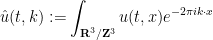
so that the system becomes

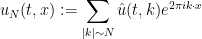
$\displaystyle \partial_t \hat u(t,k) + 2\pi \sum_{k = k_1 + k_2} (\hat u(t,k_1) \cdot ik_2) \hat u(t,k_2) =$

$\displaystyle - 4\pi^2 \nu |k|^2 \hat u(t,k) + 2\pi ik \hat p(t,k) + \hat f(t,k) \ \ \ \ \ (1)$

$\displaystyle k \cdot \hat u(t,k) = 0.$

We may normalise ${u}$ (and ${f}$ ) to have mean zero, so that ${\hat u(t,0)=0}$ . Then we introduce the dyadic energies

$\displaystyle E_N(t) := \sum_{|k| \sim N} |\hat u(t,k)|^2$

where ${N \geq 1}$ ranges over the powers of two, and ${|k| \sim N}$ is shorthand for ${N \leq |k| < 2N}$ . Taking the inner product of (1) with ${\hat u(t,k)}$ , we obtain the energy flow equation

$\displaystyle \partial_t E_N = \sum_{N_1,N_2} \Pi_{N,N_1,N_2} - D_N + F_N \ \ \ \ \ (2)$

where ${N_1,N_2}$ range over powers of two, ${\Pi_{N,N_1,N_2}}$ is the energy flow rate

$\displaystyle \Pi_{N,N_1,N_2} := -2\pi \sum_{k=k_1+k_2: |k| \sim N, |k_1| \sim N_1, |k_2| \sim N_2}$

$\displaystyle (\hat u(t,k_1) \cdot ik_2) (\hat u(t,k) \cdot \hat u(t,k_2)),$

${D_N}$ is the energy dissipation rate

$\displaystyle D_N := 4\pi^2 \nu \sum_{|k| \sim N} |k|^2 |\hat u(t,k)|^2$

and ${F_N}$ is the energy injection rate

$\displaystyle F_N := \sum_{|k| \sim N} \hat u(t,k) \cdot \hat f(t,k).$

The Navier-Stokes equations are notoriously difficult to solve in general. Despite this, Kolmogorov in 1941 was able to give a convincing heuristic argument for what the distribution of the dyadic energies ${E_N}$ should become over long times, assuming that some sort of distributional steady state is reached. It is common to present this argument in the form of dimensional analysis, but one can also give a more “first principles” form Kolmogorov’s argument, which I will do here. Heuristically, one can divide the frequency scales ${N}$ into three regimes:

The injection regime in which the energy injection rate ${F_N}$ dominates the right-hand side of (2);
The energy flow regime in which the flow rates ${\Pi_{N,N_1,N_2}}$ dominate the right-hand side of (2); and
The dissipation regime in which the dissipation ${D_N}$ dominates the right-hand side of (2).

If we assume a fairly steady and smooth forcing term ${f}$ , then ${\hat f}$ will be supported on the low frequency modes ${k=O(1)}$ , and so we heuristically expect the injection regime to consist of the low scales ${N=O(1)}$ . Conversely, if we take the viscosity ${\nu}$ to be small, we expect the dissipation regime to only occur for very large frequencies ${N}$ , with the energy flow regime occupying the intermediate frequencies.

We can heuristically predict the dividing line between the energy flow regime. Of all the flow rates ${\Pi_{N,N_1,N_2}}$ , it turns out in practice that the terms in which ${N_1,N_2 = N+O(1)}$ (i.e., interactions between comparable scales, rather than widely separated scales) will dominate the other flow rates, so we will focus just on these terms. It is convenient to return back to physical space, decomposing the velocity field ${u}$ into Littlewood-Paley components

$\displaystyle u_N(t,x) := \sum_{|k| \sim N} \hat u(t,k) e^{2\pi i k \cdot x}$

of the velocity field ${u(t,x)}$ at frequency ${N}$ . By Plancherel’s theorem, this field will have an ${L^2}$ norm of ${E_N(t)^{1/2}}$ , and as a naive model of turbulence we expect this field to be spread out more or less uniformly on the torus, so we have the heuristic

$\displaystyle |u_N(t,x)| = O( E_N(t)^{1/2} ),$

and a similar heuristic applied to ${\nabla u_N}$ gives

$\displaystyle |\nabla u_N(t,x)| = O( N E_N(t)^{1/2} ).$

(One can consider modifications of the Kolmogorov model in which ${u_N}$ is concentrated on a lower-dimensional subset of the three-dimensional torus, leading to some changes in the numerology below, but we will not consider such variants here.) Since

$\displaystyle \Pi_{N,N_1,N_2} = - \int_{{\bf R}^3/{\bf Z}^3} u_N \cdot ( (u_{N_1} \cdot \nabla) u_{N_2} )\ dx$

we thus arrive at the heuristic

$\displaystyle \Pi_{N,N_1,N_2} = O( N_2 E_N^{1/2} E_{N_1}^{1/2} E_{N_2}^{1/2} ).$

Of course, there is the possibility that due to significant cancellation, the energy flow is significantly less than ${O( N E_N(t)^{3/2} )}$ , but we will assume that cancellation effects are not that significant, so that we typically have

$\displaystyle \Pi_{N,N_1,N_2} \sim N_2 E_N^{1/2} E_{N_1}^{1/2} E_{N_2}^{1/2} \ \ \ \ \ (3)$

or (assuming that ${E_N}$ does not oscillate too much in ${N}$ , and ${N_1,N_2}$ are close to ${N}$ )

$\displaystyle \Pi_{N,N_1,N_2} \sim N E_N^{3/2}.$

On the other hand, we clearly have

$\displaystyle D_N \sim \nu N^2 E_N.$

We thus expect to be in the dissipation regime when

$\displaystyle N \gtrsim \nu^{-1} E_N^{1/2} \ \ \ \ \ (4)$

and in the energy flow regime when

$\displaystyle 1 \lesssim N \lesssim \nu^{-1} E_N^{1/2}. \ \ \ \ \ (5)$

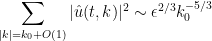
Now we study the energy flow regime further. We assume a “statistically scale-invariant” dynamics in this regime, in particular assuming a power law

$\displaystyle E_N \sim A N^{-\alpha} \ \ \ \ \ (6)$

for some ${A,\alpha > 0}$ . From (3), we then expect an average asymptotic of the form

$\displaystyle \Pi_{N,N_1,N_2} \approx A^{3/2} c_{N,N_1,N_2} (N N_1 N_2)^{1/3 - \alpha/2} \ \ \ \ \ (7)$

for some structure constants ${c_{N,N_1,N_2} \sim 1}$ that depend on the exact nature of the turbulence; here we have replaced the factor ${N_2}$ by the comparable term ${(N N_1 N_2)^{1/3}}$ to make things more symmetric. In order to attain a steady state in the energy flow regime, we thus need a cancellation in the structure constants:

$\displaystyle \sum_{N_1,N_2} c_{N,N_1,N_2} (N N_1 N_2)^{1/3 - \alpha/2} \approx 0. \ \ \ \ \ (8)$

On the other hand, if one is assuming statistical scale invariance, we expect the structure constants to be scale-invariant (in the energy flow regime), in that

$\displaystyle c_{\lambda N, \lambda N_1, \lambda N_2} = c_{N,N_1,N_2} \ \ \ \ \ (9)$

for dyadic ${\lambda > 0}$ . Also, since the Euler equations conserve energy, the energy flows ${\Pi_{N,N_1,N_2}}$ symmetrise to zero,

$\displaystyle \Pi_{N,N_1,N_2} + \Pi_{N,N_2,N_1} + \Pi_{N_1,N,N_2} + \Pi_{N_1,N_2,N} + \Pi_{N_2,N,N_1} + \Pi_{N_2,N_1,N} = 0,$

which from (7) suggests a similar cancellation among the structure constants

$\displaystyle c_{N,N_1,N_2} + c_{N,N_2,N_1} + c_{N_1,N,N_2} + c_{N_1,N_2,N} + c_{N_2,N,N_1} + c_{N_2,N_1,N} \approx 0.$

Combining this with the scale-invariance (9), we see that for fixed ${N}$ , we may organise the structure constants ${c_{N,N_1,N_2}}$ for dyadic ${N_1,N_2}$ into sextuples which sum to zero (including some degenerate tuples of order less than six). This will automatically guarantee the cancellation (8) required for a steady state energy distribution, provided that

$\displaystyle \frac{1}{3} - \frac{\alpha}{2} = 0$

or in other words

$\displaystyle \alpha = \frac{2}{3};$

for any other value of ${\alpha}$ , there is no particular reason to expect this cancellation (8) to hold. Thus we are led to the heuristic conclusion that the most stable power law distribution for the energies ${E_N}$ is the ${2/3}$ law

$\displaystyle E_N \sim A N^{-2/3} \ \ \ \ \ (10)$

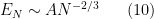
or in terms of shell energies, we have the famous Kolmogorov 5/3 law

$\displaystyle \sum_{|k| = k_0 + O(1)} |\hat u(t,k)|^2 \sim A k_0^{-5/3}.$

Given that frequency interactions tend to cascade from low frequencies to high (if only because there are so many more high frequencies than low ones), the above analysis predicts a stablising effect around this power law: scales at which a law (6) holds for some ${\alpha > 2/3}$ are likely to lose energy in the near-term, while scales at which a law (6) hold for some ${\alpha< 2/3}$ are conversely expected to gain energy, thus nudging the exponent of power law towards ${2/3}$ .

We can solve for ${A}$ in terms of energy dissipation as follows. If we let ${N_*}$ be the frequency scale demarcating the transition from the energy flow regime (5) to the dissipation regime (4), we have

$\displaystyle N_* \sim \nu^{-1} E_{N_*}$

and hence by (10)

$\displaystyle N_* \sim \nu^{-1} A N_*^{-2/3}.$

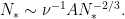
On the other hand, if we let ${\epsilon := D_{N_*}}$ be the energy dissipation at this scale ${N_*}$ (which we expect to be the dominant scale of energy dissipation), we have

$\displaystyle \epsilon \sim \nu N_*^2 E_N \sim \nu N_*^2 A N_*^{-2/3}.$

Some simple algebra then lets us solve for ${A}$ and ${N_*}$ as

$\displaystyle N_* \sim (\frac{\epsilon}{\nu^3})^{1/4}$

and

$\displaystyle A \sim \epsilon^{2/3}.$

Thus, we have the Kolmogorov prediction

$\displaystyle \sum_{|k| = k_0 + O(1)} |\hat u(t,k)|^2 \sim \epsilon^{2/3} k_0^{-5/3}$

for

$\displaystyle 1 \lesssim k_0 \lesssim (\frac{\epsilon}{\nu^3})^{1/4}$

with energy dissipation occuring at the high end ${k_0 \sim (\frac{\epsilon}{\nu^3})^{1/4}}$ of this scale, which is counterbalanced by the energy injection at the low end ${k_0 \sim 1}$ of the scale.

Finite time blowup for an averaged three-dimensional Navier-Stokes equation

4 February, 2014 in math.AP, math.CA, paper | Tags: dyadic models, finite time blowup, Navier-Stokes equations | by Terence Tao | 197 comments

I’ve just uploaded to the arXiv the paper “Finite time blowup for an averaged three-dimensional Navier-Stokes equation“, submitted to J. Amer. Math. Soc.. The main purpose of this paper is to formalise the “supercriticality barrier” for the global regularity problem for the Navier-Stokes equation, which roughly speaking asserts that it is not possible to establish global regularity by any “abstract” approach which only uses upper bound function space estimates on the nonlinear part of the equation, combined with the energy identity. This is done by constructing a modification of the Navier-Stokes equations with a nonlinearity that obeys essentially all of the function space estimates that the true Navier-Stokes nonlinearity does, and which also obeys the energy identity, but for which one can construct solutions that blow up in finite time. Results of this type had been previously established by Montgomery-Smith, Gallagher-Paicu, and Li-Sinai for variants of the Navier-Stokes equation without the energy identity, and by Katz-Pavlovic and by Cheskidov for dyadic analogues of the Navier-Stokes equations in five and higher dimensions that obeyed the energy identity (see also the work of Plechac and Sverak and of Hou and Lei that also suggest blowup for other Navier-Stokes type models obeying the energy identity in five and higher dimensions), but to my knowledge this is the first blowup result for a Navier-Stokes type equation in three dimensions that also obeys the energy identity. Intriguingly, the method of proof in fact hints at a possible route to establishing blowup for the true Navier-Stokes equations, which I am now increasingly inclined to believe is the case (albeit for a very small set of initial data).

To state the results more precisely, recall that the Navier-Stokes equations can be written in the form

$\displaystyle \partial_t u + (u \cdot \nabla) u = \nu \Delta u + \nabla p$

for a divergence-free velocity field ${u}$ and a pressure field ${p}$ , where ${\nu>0}$ is the viscosity, which we will normalise to be one. We will work in the non-periodic setting, so the spatial domain is ${{\bf R}^3}$ , and for sake of exposition I will not discuss matters of regularity or decay of the solution (but we will always be working with strong notions of solution here rather than weak ones). Applying the Leray projection ${P}$ to divergence-free vector fields to this equation, we can eliminate the pressure, and obtain an evolution equation

$\displaystyle \partial_t u = \Delta u + B(u,u) \ \ \ \ \ (1)$

purely for the velocity field, where ${B}$ is a certain bilinear operator on divergence-free vector fields (specifically, ${B(u,v) = -\frac{1}{2} P( (u \cdot \nabla) v + (v \cdot \nabla) u)}$ . The global regularity problem for Navier-Stokes is then equivalent to the global regularity problem for the evolution equation (1).

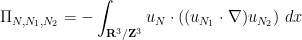
An important feature of the bilinear operator ${B}$ appearing in (1) is the cancellation law

$\displaystyle \langle B(u,u), u \rangle = 0$

(using the ${L^2}$ inner product on divergence-free vector fields), which leads in particular to the fundamental energy identity

$\displaystyle \frac{1}{2} \int_{{\bf R}^3} |u(T,x)|^2\ dx + \int_0^T \int_{{\bf R}^3} |\nabla u(t,x)|^2\ dx dt = \frac{1}{2} \int_{{\bf R}^3} |u(0,x)|^2\ dx.$

This identity (and its consequences) provide essentially the only known a priori bound on solutions to the Navier-Stokes equations from large data and arbitrary times. Unfortunately, as discussed in this previous post, the quantities controlled by the energy identity are supercritical with respect to scaling, which is the fundamental obstacle that has defeated all attempts to solve the global regularity problem for Navier-Stokes without any additional assumptions on the data or solution (e.g. perturbative hypotheses, or a priori control on a critical norm such as the ${L^\infty_t L^3_x}$ norm).

Our main result is then (slightly informally stated) as follows

Theorem 1 There exists an averaged version ${\tilde B}$ of the bilinear operator ${B}$ , of the form

$\displaystyle \tilde B(u,v) := \int_\Omega m_{3,\omega}(D) Rot_{3,\omega}$

$\displaystyle B( m_{1,\omega}(D) Rot_{1,\omega} u, m_{2,\omega}(D) Rot_{2,\omega} v )\ d\mu(\omega)$

for some probability space ${(\Omega, \mu)}$ , some spatial rotation operators ${Rot_{i,\omega}}$ for ${i=1,2,3}$ , and some Fourier multipliers ${m_{i,\omega}}$ of order ${0}$ , for which one still has the cancellation law

$\displaystyle \langle \tilde B(u,u), u \rangle = 0$

and for which the averaged Navier-Stokes equation

$\displaystyle \partial_t u = \Delta u + \tilde B(u,u) \ \ \ \ \ (2)$

admits solutions that blow up in finite time.

(There are some integrability conditions on the Fourier multipliers ${m_{i,\omega}}$ required in the above theorem in order for the conclusion to be non-trivial, but I am omitting them here for sake of exposition.)

Because spatial rotations and Fourier multipliers of order ${0}$ are bounded on most function spaces, ${\tilde B}$ automatically obeys almost all of the upper bound estimates that ${B}$ does. Thus, this theorem blocks any attempt to prove global regularity for the true Navier-Stokes equations which relies purely on the energy identity and on upper bound estimates for the nonlinearity; one must use some additional structure of the nonlinear operator ${B}$ which is not shared by an averaged version ${\tilde B}$ . Such additional structure certainly exists – for instance, the Navier-Stokes equation has a vorticity formulation involving only differential operators rather than pseudodifferential ones, whereas a general equation of the form (2) does not. However, “abstract” approaches to global regularity generally do not exploit such structure, and thus cannot be used to affirmatively answer the Navier-Stokes problem.

It turns out that the particular averaged bilinear operator ${B}$ that we will use will be a finite linear combination of local cascade operators, which take the form

$\displaystyle C(u,v) := \sum_{n \in {\bf Z}} (1+\epsilon_0)^{5n/2} \langle u, \psi_{1,n} \rangle \langle v, \psi_{2,n} \rangle \psi_{3,n}$

where ${\epsilon_0>0}$ is a small parameter, ${\psi_1,\psi_2,\psi_3}$ are Schwartz vector fields whose Fourier transform is supported on an annulus, and ${\psi_{i,n}(x) := (1+\epsilon_0)^{3n/2} \psi_i( (1+\epsilon_0)^n x)}$ is an ${L^2}$ -rescaled version of ${\psi_i}$ (basically a “wavelet” of wavelength about ${(1+\epsilon_0)^{-n}}$ centred at the origin). Such operators were essentially introduced by Katz and Pavlovic as dyadic models for ${B}$ ; they have the essentially the same scaling property as ${B}$ (except that one can only scale along powers of ${1+\epsilon_0}$ , rather than over all positive reals), and in fact they can be expressed as an average of ${B}$ in the sense of the above theorem, as can be shown after a somewhat tedious amount of Fourier-analytic symbol manipulations.

If we consider nonlinearities ${\tilde B}$ which are a finite linear combination of local cascade operators, then the equation (2) more or less collapses to a system of ODE in certain “wavelet coefficients” of ${u}$ . The precise ODE that shows up depends on what precise combination of local cascade operators one is using. Katz and Pavlovic essentially considered a single cascade operator together with its “adjoint” (needed to preserve the energy identity), and arrived (more or less) at the system of ODE

$\displaystyle \partial_t X_n = - (1+\epsilon_0)^{2n} X_n + (1+\epsilon_0)^{\frac{5}{2}(n-1)} X_{n-1}^2 - (1+\epsilon_0)^{\frac{5}{2} n} X_n X_{n+1} \ \ \ \ \ (3)$

where ${X_n: [0,T] \rightarrow {\bf R}}$ are scalar fields for each integer ${n}$ . (Actually, Katz-Pavlovic worked with a technical variant of this particular equation, but the differences are not so important for this current discussion.) Note that the quadratic terms on the RHS carry a higher exponent of ${1+\epsilon_0}$ than the dissipation term; this reflects the supercritical nature of this evolution (the energy ${\frac{1}{2} \sum_n X_n^2}$ is monotone decreasing in this flow, so the natural size of ${X_n}$ given the control on the energy is ${O(1)}$ ). There is a slight technical issue with the dissipation if one wishes to embed (3) into an equation of the form (2), but it is minor and I will not discuss it further here.

In principle, if the ${X_n}$ mode has size comparable to ${1}$ at some time ${t_n}$ , then energy should flow from ${X_n}$ to ${X_{n+1}}$ at a rate comparable to ${(1+\epsilon_0)^{\frac{5}{2} n}}$ , so that by time ${t_{n+1} \approx t_n + (1+\epsilon_0)^{-\frac{5}{2} n}}$ or so, most of the energy of ${X_n}$ should have drained into the ${X_{n+1}}$ mode (with hardly any energy dissipated). Since the series ${\sum_{n \geq 1} (1+\epsilon_0)^{-\frac{5}{2} n}}$ is summable, this suggests finite time blowup for this ODE as the energy races ever more quickly to higher and higher modes. Such a scenario was indeed established by Katz and Pavlovic (and refined by Cheskidov) if the dissipation strength ${(1+\epsilon)^{2n}}$ was weakened somewhat (the exponent ${2}$ has to be lowered to be less than ${\frac{5}{3}}$ ). As mentioned above, this is enough to give a version of Theorem 1 in five and higher dimensions.

On the other hand, it was shown a few years ago by Barbato, Morandin, and Romito that (3) in fact admits global smooth solutions (at least in the dyadic case ${\epsilon_0=1}$ , and assuming non-negative initial data). Roughly speaking, the problem is that as energy is being transferred from ${X_n}$ to ${X_{n+1}}$ , energy is also simultaneously being transferred from ${X_{n+1}}$ to ${X_{n+2}}$ , and as such the solution races off to higher modes a bit too prematurely, without absorbing all of the energy from lower modes. This weakens the strength of the blowup to the point where the moderately strong dissipation in (3) is enough to kill the high frequency cascade before a true singularity occurs. Because of this, the original Katz-Pavlovic model cannot quite be used to establish Theorem 1 in three dimensions. (Actually, the original Katz-Pavlovic model had some additional dispersive features which allowed for another proof of global smooth solutions, which is an unpublished result of Nazarov.)

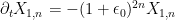
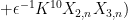
To get around this, I had to “engineer” an ODE system with similar features to (3) (namely, a quadratic nonlinearity, a monotone total energy, and the indicated exponents of ${(1+\epsilon_0)}$ for both the dissipation term and the quadratic terms), but for which the cascade of energy from scale ${n}$ to scale ${n+1}$ was not interrupted by the cascade of energy from scale ${n+1}$ to scale ${n+2}$ . To do this, I needed to insert a delay in the cascade process (so that after energy was dumped into scale ${n}$ , it would take some time before the energy would start to transfer to scale ${n+1}$ ), but the process also needed to be abrupt (once the process of energy transfer started, it needed to conclude very quickly, before the delayed transfer for the next scale kicked in). It turned out that one could build a “quadratic circuit” out of some basic “quadratic gates” (analogous to how an electrical circuit could be built out of basic gates such as amplifiers or resistors) that achieved this task, leading to an ODE system essentially of the form

$\displaystyle \partial_t X_{1,n} = - (1+\epsilon_0)^{2n} X_{1,n}$

$\displaystyle + (1+\epsilon_0)^{5n/2} (- \epsilon^{-2} X_{3,n} X_{4,n} - \epsilon X_{1,n} X_{2,n} - \epsilon^2 \exp(-K^{10}) X_{1,n} X_{3,n}$

$\displaystyle + K X_{4,n-1}^2)$

$\displaystyle \partial_t X_{2,n} = - (1+\epsilon_0)^{2n} X_{2,n} + (1+\epsilon_0)^{5n/2} (\epsilon X_{1,n}^2 - \epsilon^{-1} K^{10} X_{3,n}^2)$

$\displaystyle \partial_t X_{3,n} = - (1+\epsilon_0)^{2n} X_{3,n} + (1+\epsilon_0)^{5n/2} (\epsilon^2 \exp(-K^{10}) X_{1,n}^2$

$\displaystyle + \epsilon^{-1} K^{10} X_{2,n} X_{3,n} )$

$\displaystyle \partial_t X_{4,n} =- (1+\epsilon_0)^{2n} X_{4,n} + (1+\epsilon_0)^{5n/2} (\epsilon^{-2} X_{3,n} X_{1,n}$

$\displaystyle - (1+\epsilon_0)^{5/2} K X_{4,n} X_{1,n+1})$

where ${K \geq 1}$ is a suitable large parameter and ${\epsilon > 0}$ is a suitable small parameter (much smaller than ${1/K}$ ). To visualise the dynamics of such a system, I found it useful to describe this system graphically by a “circuit diagram” that is analogous (but not identical) to the circuit diagrams arising in electrical engineering:

The coupling constants here range widely from being very large to very small; in practice, this makes the ${X_{2,n}}$ and ${X_{3,n}}$ modes absorb very little energy, but exert a sizeable influence on the remaining modes. If a lot of energy is suddenly dumped into ${X_{1,n}}$ , what happens next is roughly as follows: for a moderate period of time, nothing much happens other than a trickle of energy into ${X_{2,n}}$ , which in turn causes a rapid exponential growth of ${X_{3,n}}$ (from a very low base). After this delay, ${X_{3,n}}$ suddenly crosses a certain threshold, at which point it causes ${X_{1,n}}$ and ${X_{4,n}}$ to exchange energy back and forth with extreme speed. The energy from ${X_{4,n}}$ then rapidly drains into ${X_{1,n+1}}$ , and the process begins again (with a slight loss in energy due to the dissipation). If one plots the total energy ${E_n := \frac{1}{2} ( X_{1,n}^2 + X_{2,n}^2 + X_{3,n}^2 + X_{4,n}^2 )}$ as a function of time, it looks schematically like this:

As in the previous heuristic discussion, the time between cascades from one frequency scale to the next decay exponentially, leading to blowup at some finite time ${T}$ . (One could describe the dynamics here as being similar to the famous “lighting the beacons” scene in the Lord of the Rings movies, except that (a) as each beacon gets ignited, the previous one is extinguished, as per the energy identity; (b) the time between beacon lightings decrease exponentially; and (c) there is no soundtrack.)

There is a real (but remote) possibility that this sort of construction can be adapted to the true Navier-Stokes equations. The basic blowup mechanism in the averaged equation is that of a von Neumann machine, or more precisely a construct (built within the laws of the inviscid evolution ${\partial_t u = \tilde B(u,u)}$ ) that, after some time delay, manages to suddenly create a replica of itself at a finer scale (and to largely erase its original instantiation in the process). In principle, such a von Neumann machine could also be built out of the laws of the inviscid form of the Navier-Stokes equations (i.e. the Euler equations). In physical terms, one would have to build the machine purely out of an ideal fluid (i.e. an inviscid incompressible fluid). If one could somehow create enough “logic gates” out of ideal fluid, one could presumably build a sort of “fluid computer”, at which point the task of building a von Neumann machine appears to reduce to a software engineering exercise rather than a PDE problem (providing that the gates are suitably stable with respect to perturbations, but (as with actual computers) this can presumably be done by converting the analog signals of fluid mechanics into a more error-resistant digital form). The key thing missing in this program (in both senses of the word) to establish blowup for Navier-Stokes is to construct the logic gates within the laws of ideal fluids. (Compare with the situation for cellular automata such as Conway’s “Game of Life“, in which Turing complete computers, universal constructors, and replicators have all been built within the laws of that game.)

A correction to “Localisation and compactness properties of the Navier-Stokes global regularity problem”

7 August, 2011 in math.AP, math.MP, update | Tags: global well-posedness, Navier-Stokes equations | by Terence Tao | 23 comments

A few days ago, I released a preprint entitled “Localisation and compactness properties of the Navier-Stokes global regularity problem“, discussed in this previous blog post. As it turns out, I was somewhat impatient to finalise the paper and move on to other things, and the original preprint was still somewhat rough in places (contradicting my own advice on this matter), with a number of typos of minor to moderate severity. But a bit more seriously, I discovered on a further proofreading that there was a subtle error in a component of the argument that I had believed to be routine – namely the persistence of higher regularity for mild solutions. As a consequence, some of the implications stated in the first version were not exactly correct as stated; but they can be repaired by replacing a “bad” notion of global regularity for a certain class of data with a “good” notion. I have completed (and proofread) an updated version of the ms, which should appear at the arXiv link of the paper in a day or two (and which I have also placed at this link). (In the meantime, it is probably best not to read the original ms too carefully, as this could lead to some confusion.) I’ve also added a new section that shows that, due to this technicality, one can exhibit smooth $H^1$ initial data to the Navier-Stokes equation for which there are no smooth solutions, which superficially sounds very close to a negative solution to the global regularity problem, but is actually nothing of the sort.

Let me now describe the issue in more detail (and also to explain why I missed it previously). A standard principle in the theory of evolutionary partial differentiation equations is that regularity in space can be used to imply regularity in time. To illustrate this, consider a solution $u$ to the supercritical nonlinear wave equation

$-\partial_{tt} u + \Delta u = u^7$ (1)

for some field $u: {\bf R} \times {\bf R}^3 \to {\bf R}$ . Suppose one already knew that $u$ had some regularity in space, and in particular the $C^0_t C^2_x \cap C^1_t C^1_x$ norm of $u$ was bounded (thus $u$ and up to two spatial derivatives of $u$ were bounded). Then, by (1), we see that two time derivatives of $u$ were also bounded, and one then gets the additional regularity of $C^2_t C^0_x$ .

In a similar vein, suppose one initially knew that $u$ had the regularity $C^0_t C^3_x \cap C^1_t C^2_x$ . Then (1) soon tells us that $u$ also has the regularity $C^2_t C^1_x$ ; then, if one differentiates (1) in time to obtain

$-\partial_{ttt} u + \Delta \partial_t u = 7 u^6 \partial_t u$

one can conclude that $u$ also has the regularity of $C^3_t C^0_x$ . One can continue this process indefinitely; in particular, if one knew that $u \in C^0_t C^\infty_x \cap C^1_t C^\infty_x$ , then these sorts of manipulations show that $u$ is infinitely smooth in both space and time.

The issue that caught me by surprise is that for the Navier-Stokes equations

$\partial_t u + (u \cdot \nabla) u =\Delta u -\nabla p$ (2)

$\nabla \cdot u = 0$

(setting the forcing term $f$ equal to zero for simplicity), infinite regularity in space does not automatically imply infinite regularity in time, even if one assumes the initial data lies in a standard function space such as the Sobolev space $H^1_x({\bf R}^3)$ . The problem lies with the pressure term $p$ , which is recovered from the velocity via the elliptic equation

$\Delta p = -\nabla^2 \cdot (u \otimes u)$ (3)

that can be obtained by taking the divergence of (2). This equation is solved by a non-local integral operator:

$\displaystyle p(t,x) = \int_{{\bf R}^3} \frac{\nabla^2 \cdot (u \otimes u)(t,y)}{4\pi |x-y|}\ dy.$

If, say, $u$ lies in $H^1_x({\bf R}^3)$ , then there is no difficulty establishing a bound on $p$ in terms of $u$ (for instance, one can use singular integral theory and Sobolev embedding to place $p$ in $L^3_x({\bf R}^3)$ . However, one runs into difficulty when trying to compute time derivatives of $p$ . Differentiating (3) once, one gets

$\Delta \partial_t p = -2\nabla^2 \cdot (u \otimes \partial_t u)$ .

At the regularity of $H^1$ , one can still (barely) control this quantity by using (2) to expand out $\partial_t u$ and using some integration by parts. But when one wishes to compute a second time derivative of the pressure, one obtains (after integration by parts) an expansion of the form

$\Delta \partial_{tt} p = -4\nabla^2 \cdot (\Delta u \otimes \Delta u) + \ldots$

and now there is not enough regularity on $u$ available to get any control on $\partial_{tt} p$ , even if one assumes that $u$ is smooth. Indeed, following this observation, I was able to show that given generic smooth $H^1$ data, the pressure $p$ will instantaneously fail to be $C^2$ in time, and thence (by (2)) the velocity will instantaneously fail to be $C^3$ in time. (Switching to the vorticity formulation buys one further degree of time differentiability, but does not fully eliminate the problem; the vorticity $\omega$ will fail to be $C^4$ in time. Switching to material coordinates seems to makes things very slightly better, but I believe there is still a breakdown of time regularity in these coordinates also.)

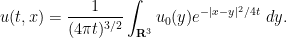
For later times t>0 (and assuming homogeneous data f=0 for simplicity), this issue no longer arises, because of the instantaneous smoothing effect of the Navier-Stokes flow, which for instance will upgrade $H^1_x$ regularity to $H^\infty_x$ regularity instantaneously. It is only the initial time at which some time irregularity can occur.

This breakdown of regularity does not actually impact the original formulation of the Clay Millennium Prize problem, though, because in that problem the initial velocity is required to be Schwartz class (so all derivatives are rapidly decreasing). In this class, the regularity theory works as expected; if one has a solution which already has some reasonable regularity (e.g. a mild $H^1$ solution) and the data is Schwartz, then the solution will be smooth in spacetime. (Another class where things work as expected is when the vorticity is Schwartz; in such cases, the solution remains smooth in both space and time (for short times, at least), and the Schwartz nature of the vorticity is preserved (because the vorticity is subject to fewer non-local effects than the velocity, as it is not directly affected by the pressure).)

This issue means that one of the implications in the original paper (roughly speaking, that global regularity for Schwartz data implies global regularity for smooth $H^1$ data) is not correct as stated. But this can be fixed by weakening the notion of global regularity in the latter setting, by limiting the amount of time differentiability available at the initial time. More precisely, call a solution $u: [0,T] \times {\bf R}^3 \to {\bf R}^3$ and $p: [0,T] \times {\bf R}^3 \to {\bf R}$ almost smooth if

$u$ and $p$ are smooth on the half-open slab $(0,T] \times {\bf R}^3$ ; and
For every $k \geq 0$ , $\nabla^k_x u, \nabla^k_x p, \nabla^x_u \partial_t u$ exist and are continuous on the full slab $[0,T] \times {\bf R}^3$ .

Thus, an almost smooth solution is the same concept as a smooth solution, except that at time zero, the velocity field is only $C^1_t C^\infty_x$ , and the pressure field is only $C^0_t C^\infty_x$ . This is still enough regularity to interpret the Navier-Stokes equation (2) in a classical manner, but falls slightly short of full smoothness.

(I had already introduced this notion of almost smoothness in the more general setting of smooth finite energy solutions in the first draft of this paper, but had failed to realise that it was also necessary in the smooth $H^1$ setting also.)

One can now “fix” the global regularity conjectures for Navier-Stokes in the smooth $H^1$ or smooth finite energy setting by requiring the solutions to merely be almost smooth instead of smooth. Once one does so, the results in my paper then work as before: roughly speaking, if one knows that Schwartz data produces smooth solutions, one can conclude that smooth $H^1$ or smooth finite energy data produces almost smooth solutions (and the paper now contains counterexamples to show that one does not always have smooth solutions in this category).

The diagram of implications between conjectures has been adjusted to reflect this issue, and now reads as follows:

Localisation and compactness properties of the Navier-Stokes global regularity problem

4 August, 2011 in math.AP, math.MP, paper | Tags: concentration compactness, energy estimates, global well-posedness, homogenisation, localisation, Navier-Stokes equations | by Terence Tao | 11 comments

I’ve just uploaded to the arXiv my paper “Localisation and compactness properties of the Navier-Stokes global regularity problem“, submitted to Analysis and PDE. This paper concerns the global regularity problem for the Navier-Stokes system of equations

$\displaystyle \partial_t u + (u \cdot \nabla) u = \Delta u - \nabla p + f \ \ \ \ \ (1)$

$\displaystyle \nabla \cdot u = 0 \ \ \ \ \ (2)$

$\displaystyle u(0,\cdot) = u_0 \ \ \ \ \ (3)$

in three dimensions. Thus, we specify initial data ${(u_0,f,T)}$ , where ${0 < T < \infty}$ is a time, ${u_0: {\bf R}^3 \rightarrow {\bf R}^3}$ is the initial velocity field (which, in order to be compatible with (2), (3), is required to be divergence-free), ${f: [0,T] \times {\bf R}^3 \rightarrow {\bf R}^3}$ is the forcing term, and then seek to extend this initial data to a solution ${(u,p,u_0,f,T)}$ with this data, where the velocity field ${u: [0,T] \times {\bf R}^3 \rightarrow {\bf R}^3}$ and pressure term ${p: [0,T] \times {\bf R}^3 \rightarrow {\bf R}}$ are the unknown fields.

Roughly speaking, the global regularity problem asserts that given every smooth set of initial data ${(u_0,f,T)}$ , there exists a smooth solution ${(u,p,u_0,f,T)}$ to the Navier-Stokes equation with this data. However, this is not a good formulation of the problem because it does not exclude the possibility that one or more of the fields ${u_0, f, u, p}$ grows too fast at spatial infinity. This problem is evident even for the much simpler heat equation

$\displaystyle \partial_t u = \Delta u$

$\displaystyle u(0,\cdot) = u_0.$

As long as one has some mild conditions at infinity on the smooth initial data ${u_0: {\bf R}^3 \rightarrow {\bf R}}$ (e.g. polynomial growth at spatial infinity), then one can solve this equation using the fundamental solution of the heat equation:

$\displaystyle u(t,x) = \frac{1}{(4\pi t)^{3/2}} \int_{{\bf R}^3} u_0(y) e^{-|x-y|^2/4t}\ dy.$

If furthermore ${u}$ is a tempered distribution, one can use Fourier-analytic methods to show that this is the unique solution to the heat equation with this data. But once one allows sufficiently rapid growth at spatial infinity, existence and uniqueness can break down. Consider for instance the backwards heat kernel

$\displaystyle u(t,x) = \frac{1}{(4\pi(T-t))^{3/2}} e^{|x|^2/(T-t)}$

for some ${T>0}$ , which is smooth (albeit exponentially growing) at time zero, and is a smooth solution to the heat equation for ${0 \leq t < T}$ , but develops a dramatic singularity at time ${t=T}$ . A famous example of Tychonoff from 1935, based on a power series construction, also shows that uniqueness for the heat equation can also fail once growth conditions are removed. An explicit example of non-uniqueness for the heat equation is given by the contour integral

$\displaystyle u(t,x_1,x_2,x_3) = \int_\gamma \exp(e^{\pi i/4} x_1 z + e^{5\pi i/8} z^{3/2} - itz^2)\ dz$

where ${\gamma}$ is the ${L}$ -shaped contour consisting of the positive real axis and the upper imaginary axis, with ${z^{3/2}}$ being interpreted with the standard branch (with cut on the negative axis). One can show by contour integration that this function solves the heat equation and is smooth (but rapidly growing at infinity), and vanishes for ${t<0}$ , but is not identically zero for ${t>0}$ .

Thus, in order to obtain a meaningful (and physically realistic) problem, one needs to impose some decay (or at least limited growth) hypotheses on the data ${u_0,f}$ and solution ${u,p}$ in addition to smoothness. For the data, one can impose a variety of such hypotheses, including the following:

(Finite energy data) One has ${\|u_0\|_{L^2_x({\bf R}^3)} < \infty}$ and ${\| f \|_{L^\infty_t L^2_x([0,T] \times {\bf R}^3)} < \infty}$ .
( ${H^1}$ data) One has ${\|u_0\|_{H^1_x({\bf R}^3)} < \infty}$ and ${\| f \|_{L^\infty_t H^1_x([0,T] \times {\bf R}^3)} < \infty}$ .
(Schwartz data) One has ${\sup_{x \in {\bf R}^3} ||x|^m \nabla_x^k u_0(x)| < \infty}$ and ${\sup_{(t,x) \in [0,T] \times {\bf R}^3} ||x|^m \nabla_x^k \partial_t^l f(t,x)| < \infty}$ for all ${m,k,l \geq 0}$ .
(Periodic data) There is some ${0 < L < \infty}$ such that ${u_0(x+Lk) = u_0(x)}$ and ${f(t,x+Lk) = f(t,x)}$ for all ${(t,x) \in [0,T] \times {\bf R}^3}$ and ${k \in {\bf Z}^3}$ .
(Homogeneous data) ${f=0}$ .

Note that smoothness alone does not necessarily imply finite energy, ${H^1}$ , or the Schwartz property. For instance, the (scalar) function ${u(x) = \exp( i |x|^{10} ) (1+|x|)^{-2}}$ is smooth and finite energy, but not in ${H^1}$ or Schwartz. Periodicity is of course incompatible with finite energy, ${H^1}$ , or the Schwartz property, except in the trivial case when the data is identically zero.

Similarly, one can impose conditions at spatial infinity on the solution, such as the following:

(Finite energy solution) One has ${\| u \|_{L^\infty_t L^2_x([0,T] \times {\bf R}^3)} < \infty}$ .
( ${H^1}$ solution) One has ${\| u \|_{L^\infty_t H^1_x([0,T] \times {\bf R}^3)} < \infty}$ and ${\| u \|_{L^2_t H^2_x([0,T] \times {\bf R}^3)} < \infty}$ .
(Partially periodic solution) There is some ${0 < L < \infty}$ such that ${u(t,x+Lk) = u(t,x)}$ for all ${(t,x) \in [0,T] \times {\bf R}^3}$ and ${k \in {\bf Z}^3}$ .
(Fully periodic solution) There is some ${0 < L < \infty}$ such that ${u(t,x+Lk) = u(t,x)}$ and ${p(t,x+Lk) = p(t,x)}$ for all ${(t,x) \in [0,T] \times {\bf R}^3}$ and ${k \in {\bf Z}^3}$ .

(The ${L^2_t H^2_x}$ component of the ${H^1}$ solution is for technical reasons, and should not be paid too much attention for this discussion.) Note that we do not consider the notion of a Schwartz solution; as we shall see shortly, this is too restrictive a concept of solution to the Navier-Stokes equation.

Finally, one can downgrade the regularity of the solution down from smoothness. There are many ways to do so; two such examples include

( ${H^1}$ mild solutions) The solution is not smooth, but is ${H^1}$ (in the preceding sense) and solves the equation (1) in the sense that the Duhamel formula
$\displaystyle u(t) = e^{t\Delta} u_0 + \int_0^t e^{(t-t')\Delta} (-(u\cdot\nabla) u-\nabla p+f)(t')\ dt'$

holds.
(Leray-Hopf weak solution) The solution ${u}$ is not smooth, but lies in ${L^\infty_t L^2_x \cap L^2_t H^1_x}$ , solves (1) in the sense of distributions (after rewriting the system in divergence form), and obeys an energy inequality.

Finally, one can ask for two types of global regularity results on the Navier-Stokes problem: a qualitative regularity result, in which one merely provides existence of a smooth solution without any explicit bounds on that solution, and a quantitative regularity result, which provides bounds on the solution in terms of the initial data, e.g. a bound of the form

$\displaystyle \| u \|_{L^\infty_t H^1_x([0,T] \times {\bf R}^3)} \leq F( \|u_0\|_{H^1_x({\bf R}^3)} + \|f\|_{L^\infty_t H^1_x([0,T] \times {\bf R}^3)}, T )$

for some function ${F: {\bf R}^+ \times {\bf R}^+ \rightarrow {\bf R}^+}$ . One can make a further distinction between local quantitative results, in which ${F}$ is allowed to depend on ${T}$ , and global quantitative results, in which there is no dependence on ${T}$ (the latter is only reasonable though in the homogeneous case, or if ${f}$ has some decay in time).

By combining these various hypotheses and conclusions, we see that one can write down quite a large number of slightly different variants of the global regularity problem. In the official formulation of the regularity problem for the Clay Millennium prize, a positive correct solution to either of the following two problems would be accepted for the prize:

Conjecture 1.4 (Qualitative regularity for homogeneous periodic data) If ${(u_0,0,T)}$ is periodic, smooth, and homogeneous, then there exists a smooth partially periodic solution ${(u,p,u_0,0,T)}$ with this data.
Conjecture 1.3 (Qualitative regularity for homogeneous Schwartz data) If ${(u_0,0,T)}$ is Schwartz and homogeneous, then there exists a smooth finite energy solution ${(u,p,u_0,0,T)}$ with this data.

(The numbering here corresponds to the numbering in the paper.)

Furthermore, a negative correct solution to either of the following two problems would also be accepted for the prize:

Conjecture 1.6 (Qualitative regularity for periodic data) If ${(u_0,f,T)}$ is periodic and smooth, then there exists a smooth partially periodic solution ${(u,p,u_0,f,T)}$ with this data.
Conjecture 1.5 (Qualitative regularity for Schwartz data) If ${(u_0,f,T)}$ is Schwartz, then there exists a smooth finite energy solution ${(u,p,u_0,f,T)}$ with this data.

I am not announcing any major progress on these conjectures here. What my paper does study, though, is the question of whether the answer to these conjectures is somehow sensitive to the choice of formulation. For instance:

Note in the periodic formulations of the Clay prize problem that the solution is only required to be partially periodic, rather than fully periodic; thus the pressure has no periodicity hypothesis. One can ask the extent to which the above problems change if one also requires pressure periodicity.
In another direction, one can ask the extent to which quantitative formulations of the Navier-Stokes problem are stronger than their qualitative counterparts; in particular, whether it is possible that each choice of initial data in a certain class leads to a smooth solution, but with no uniform bound on that solution in terms of various natural norms of the data.
Finally, one can ask the extent to which the conjecture depends on the category of data. For instance, could it be that global regularity is true for smooth periodic data but false for Schwartz data? True for Schwartz data but false for smooth ${H^1}$ data? And so forth.

One motivation for the final question (which was posed to me by my colleague, Andrea Bertozzi) is that the Schwartz property on the initial data ${u_0}$ tends to be instantly destroyed by the Navier-Stokes flow. This can be seen by introducing the vorticity ${\omega := \nabla \times u}$ . If ${u(t)}$ is Schwartz, then from Stokes’ theorem we necessarily have vanishing of certain moments of the vorticity, for instance:

$\displaystyle \int_{{\bf R}^3} \omega_1 (x_2^2-x_3^2)\ dx = 0.$

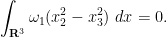
On the other hand, some integration by parts using (1) reveals that such moments are usually not preserved by the flow; for instance, one has the law

$\displaystyle \partial_t \int_{{\bf R}^3} \omega_1(t,x) (x_2^2-x_3^2)\ dx = 4\int_{{\bf R}^3} u_2(t,x) u_3(t,x)\ dx,$

and one can easily concoct examples for which the right-hand side is non-zero at time zero. This suggests that the Schwartz class may be unnecessarily restrictive for Conjecture 1.3 or Conjecture 1.5.

My paper arose out of an attempt to address these three questions, and ended up obtaining partial results in all three directions. Roughly speaking, the results that address these three questions are as follows:

(Homogenisation) If one only assumes partial periodicity instead of full periodicity, then the forcing term ${f}$ becomes irrelevant. In particular, Conjecture 1.4 and Conjecture 1.6 are equivalent.
(Concentration compactness) In the ${H^1}$ category (both periodic and nonperiodic, homogeneous or nonhomogeneous), the qualitative and quantitative formulations of the Navier-Stokes global regularity problem are essentially equivalent.
(Localisation) The (inhomogeneous) Navier-Stokes problems in the Schwartz, smooth ${H^1}$ , and finite energy categories are essentially equivalent to each other, and are also implied by the (fully) periodic version of these problems.

The first two of these families of results are relatively routine, drawing on existing methods in the literature; the localisation results though are somewhat more novel, and introduce some new local energy and local enstrophy estimates which may be of independent interest.

Broadly speaking, the moral to draw from these results is that the precise formulation of the Navier-Stokes equation global regularity problem is only of secondary importance; modulo a number of caveats and technicalities, the various formulations are close to being equivalent, and a breakthrough on any one of the formulations is likely to lead (either directly or indirectly) to a comparable breakthrough on any of the others.

This is only a caricature of the actual implications, though. Below is the diagram from the paper indicating the various formulations of the Navier-Stokes equations, and the known implications between them:

The above three streams of results are discussed in more detail below the fold.

Read the rest of this entry »

Global regularity for a logarithmically supercritical hyperdissipative Navier-Stokes equation

19 June, 2009 in math.AP, paper | Tags: logarithmically supercritical equations, Navier-Stokes equations | by Terence Tao | 35 comments

I’ve just uploaded to the arXiv my paper “Global regularity for a logarithmically supercritical hyperdissipative Navier-Stokes equation“, submitted to Analysis & PDE. It is a famous problem to establish the existence of global smooth solutions to the three-dimensional Navier-Stokes system of equations

$\partial_t u + (u \cdot \nabla) u = \Delta u - \nabla p$
$\nabla \cdot u = 0$
$u(0,x) = u_0(x)$

given smooth, compactly supported, divergence-free initial data $u_0: {\Bbb R}^3 \to {\Bbb R}^3$ .

I do not claim to have any substantial progress on this problem here. Instead, the paper makes a small observation about the hyper-dissipative version of the Navier-Stokes equations, namely

$\partial_t u + (u \cdot \nabla) u = - |\nabla|^{2\alpha} u - \nabla p$
$\nabla \cdot u = 0$
$u(0,x) = u_0(x)$

for some $\alpha > 1$ . It is a folklore result that global regularity for this equation holds for $\alpha \geq 5/4$ ; the significance of the exponent $5/4$ is that it is energy-critical, in the sense that the scaling which preserves this particular hyper-dissipative Navier-Stokes equation, also preserves the energy.

Values of $\alpha$ below $5/4$ (including, unfortunately, the case $\alpha=1$ , which is the original Navier-Stokes equation) are supercritical and thus establishing global regularity beyond the reach of most known methods (see my earlier blog post for more discussion).

A few years ago, I observed (in the case of the spherically symmetric wave equation) that this “criticality barrier” had a very small amount of flexibility to it, in that one could push a critical argument to a slightly supercritical one by exploiting spacetime integral estimates a little bit more. I realised recently that the same principle applied to hyperdissipative Navier-Stokes; here, the relevant spacetime integral estimate is the energy dissipation inequality

$\int_0^T \int_{{\Bbb R}^d} | |\nabla|^\alpha u(t,x)|^2\ dx dt \leq \frac{1}{2} \int_{{\Bbb R}^d} |u_0(x)|^2\ dx$

which ensures that the energy dissipation $a(t) := \int_{{\Bbb R}^d} | |\nabla|^\alpha u(t,x)|^2\ dx$ is locally integrable (and in fact globally integrable) in time.

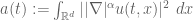
In this paper I push the global regularity results by a fraction of a logarithm from $\alpha=5/4$ towards $\alpha=1$ . For instance, the argument shows that the logarithmically supercritical equation

$\partial_t u + (u \cdot \nabla) u = - \frac{|\nabla|^{5/2}}{\log^{1/2}(2-\Delta)} u - \nabla p$ (0)
$\nabla \cdot u = 0$
$u(0,x) = u_0(x)$

admits global smooth solutions.

The argument is in fact quite simple (the paper is seven pages in length), and relies on known technology; one just applies the energy method and a logarithmically modified Sobolev inequality in the spirit of a well-known inequality of Brezis and Wainger. It looks like it will take quite a bit of effort though to improve the logarithmic factor much further.

One way to explain the tiny bit of wiggle room beyond the critical case is as follows. The standard energy method approach to the critical Navier-Stokes equation relies at one stage on Gronwall’s inequality, which among other things asserts that if a time-dependent non-negative quantity E(t) obeys the differential inequality

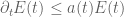
$\partial_t E(t) \leq a(t) E(t)$ (1)

and $a(t)$ was locally integrable, then E does not blow up in time; in fact, one has the inequality

$E(t) \leq E(0) \exp( \int_0^t a(s)\ ds )$ .

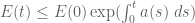
A slight modification of the argument shows that one can replace the linear inequality with a slightly superlinear inequality. For instance, the differential inequality

$\partial_t E(t) \leq a(t) E(t) \log E(t)$ (2)

also does not blow up in time; indeed, a separation of variables argument gives the explicit double-exponential bound

$E(t) \leq \exp(\exp( \int_0^t a(s)\ ds + \log \log E(0) ))$

(let’s take $E(0) > 1$ and all functions smooth, to avoid technicalities). It is this ability to go beyond Gronwall’s inequality by a little bit which is really at the heart of the logarithmically supercritical phenomenon. In the paper, I establish an inequality basically of the shape (2), where $E(t)$ is a suitably high-regularity Sobolev norm of $u(t)$ , and $a(t)$ is basically the energy dissipation mentioned earlier. The point is that the logarithmic loss of $\log(1 - \Delta)^{1/4}$ in the dissipation can eventually be converted (by a Brezis-Wainger type argument) to a logarithmic loss in the high-regularity energy, as this energy can serve as a proxy for the frequency $|\xi|$ , which in turn serves as a proxy for the Laplacian $-\Delta$ .

To put it another way, with a linear exponential growth model, such as $\partial_t E(t) = C E(t)$ , it takes a constant amount of time for E to double, and so E never becomes infinite in finite time. With an equation such as $\partial_t E(t) = C E(t) \log E(t)$ , the time taken for E to double from (say) $2^n$ to $2^{n+1}$ now shrinks to zero, but only as quickly as the harmonic series $1/n$ , so it still takes an infinite amount of time for E to blow up. But because the divergence of $\sum_n 1/n$ is logarithmically slow, the growth of E is now a double exponential rather than a single one. So there is a little bit of room to exploit between exponential growth and blowup.

Interestingly, there is a heuristic argument that suggests that the half-logarithmic loss in (0) can be widened to a full logarithmic loss, which I give below the fold.

Read the rest of this entry »

A quantitative formulation of the global regularity problem for the periodic Navier-Stokes equation

9 October, 2007 in math.AP, paper | Tags: compactness, Navier-Stokes equations | by Terence Tao | 41 comments

I have just uploaded to the arXiv my paper “A quantitative formulation of the global regularity problem for the periodic Navier-Stokes equation”, submitted to Dynamics of PDE. This is a short note on one formulation of the Clay Millennium prize problem, namely that there exists a global smooth solution to the Navier-Stokes equation on the torus $({\Bbb R}/{\Bbb Z})^3$ given any smooth divergence-free data. (I should emphasise right off the bat that I am not claiming any major breakthrough on this problem, which remains extremely challenging in my opinion.)
This problem is formulated in a qualitative way: the conjecture asserts that the velocity field $u$ stays smooth for all time, but does not ask for a quantitative bound on the smoothness of that field in terms of the smoothness of the initial data. Nevertheless, it turns out that the compactness properties of the periodic Navier-Stokes flow allow one to equate the qualitative claim with a more concrete quantitative one. More precisely, the paper shows that the following three statements are equivalent:

(Qualitative regularity conjecture) Given any smooth divergence-free data $u_0: ({\Bbb R}/{\Bbb Z})^3 \to {\Bbb R}^3$ , there exists a global smooth solution $u: [0,+\infty) \times ({\Bbb R}/{\Bbb Z})^3 \to {\Bbb R}^3$ to the Navier-Stokes equations.
(Local-in-time quantitative regularity conjecture)
Given any smooth solution $u: [0,T] \times ({\Bbb R}/{\Bbb Z})^3 \to {\Bbb R}^3$ to the Navier-Stokes equations with $0 < T \leq 1$ , one has the a priori bound $\| u(T) \|_{H^1(({\Bbb R}/{\Bbb Z})^3)} \leq F( \| u(0) \|_{H^1(({\Bbb R}/{\Bbb Z})^3)} )$ for some non-decreasing function $F:[0,+\infty) \to [0,+\infty)$ .
(Global-in-time quantitative regularity conjecture) This is the same conjecture as 2, but with the condition $0 < T \leq 1$ replaced by $0 < T < \infty$ .

It is easy to see that Conjecture 3 implies Conjecture 2, which implies Conjecture 1. By using the compactness of the local periodic Navier-Stokes flow in $H^1$ , one can show that Conjecture 1 implies Conjecture 2; and by using the energy identity (and in particular the fact that the energy dissipation is bounded) one can deduce Conjecture 3 from Conjecture 2. The argument uses only standard tools and is likely to generalise in a number of ways, which I discuss in the paper. (In particular one should be able to replace the $H^1$ norm here by any other subcritical norm.)

Read the rest of this entry »

	Aleksandar on 245C, Notes 4: Sobolev sp…
	Anonymous on Erratum for “An inverse…
	Anonymous on Erratum for “An inverse…
	Anonymous on Erratum for “An inverse…
	Anonymous on Erratum for “An inverse…
	Terence Tao on 245C, Notes 4: Sobolev sp…
	Terence Tao on 275A, Notes 3: The weak and st…
	Terence Tao on What is a gauge?
	Terence Tao on Erratum for “An inverse…
	Terence Tao on 275A, Notes 3: The weak and st…
	Terence Tao on An epsilon of room: pages from…
	Aleksandar on 245C, Notes 4: Sobolev sp…
	Anonymous on Some notes on amenability
	Anonymous on On writing
	Anonymous on 275A, Notes 3: The weak and st…

Tag Archive

Quantitative bounds for critically bounded solutions to the Navier-Stokes equations

Searching for singularities in the Navier–Stokes equations

254A, Notes 2: Weak solutions of the Navier-Stokes equations

254A, Notes 0: Physical derivation of the incompressible Euler and Navier-Stokes equations

Kolmogorov’s power law for turbulence

Finite time blowup for an averaged three-dimensional Navier-Stokes equation

A correction to “Localisation and compactness properties of the Navier-Stokes global regularity problem”

Localisation and compactness properties of the Navier-Stokes global regularity problem

Global regularity for a logarithmically supercritical hyperdissipative Navier-Stokes equation

A quantitative formulation of the global regularity problem for the periodic Navier-Stokes equation

Recent Comments

Articles by others

Diversions

Mathematics

Selected articles

Software

The sciences

Top Posts

Archives

Categories

The Polymath Blog

For commenters