
In the previous two quarters, we have been focusing largely on the “soft” side of real analysis, which is primarily concerned with “qualitative” properties such as convergence, compactness, measurability, and so forth. In contrast, we will begin this quarter with more of an emphasis on the “hard” side of real analysis, in which we study estimates and upper and lower bounds of various quantities, such as norms of functions or operators. (Of course, the two sides of analysis are closely connected to each other; an understanding of both sides and their interrelationships, are needed in order to get the broadest and most complete perspective for this subject.)
One basic tool in hard analysis is that of interpolation, which allows one to start with a hypothesis of two (or more) “upper bound” estimates, e.g. 


As is the case with many other tools in analysis, interpolation is not captured by a single “interpolation theorem”; instead, there are a family of such theorems, which can be broadly divided into two major categories, reflecting the two basic methods that underlie the principle of interpolation. The real interpolation method is based on a divide and conquer strategy: to understand how to obtain control on some expression such as 

The complex interpolation method instead proceeds by exploiting the powerful tools of complex analysis, in particular the maximum modulus principle and its relatives (such as the Phragmén-Lindelöf principle). The idea is to rewrite the estimate to be proven (e.g. 
![{\{ \sigma+it: t \in {\bf R}, \sigma \in [0,1]\}}](https://s0.wp.com/latex.php?latex=%7B%5C%7B+%5Csigma%2Bit%3A+t+%5Cin+%7B%5Cbf+R%7D%2C+%5Csigma+%5Cin+%5B0%2C1%5D%5C%7D%7D&bg=ffffff&fg=000000&s=0&c=20201002)

Despite these differences, the real and complex methods tend to give broadly similar results in practice, especially if one is willing to ignore constant losses in the estimates or epsilon losses in the exponents.
The theory of both real and complex interpolation can be studied abstractly, in general normed or quasi-normed spaces; see e.g. this book for a detailed treatment. However in these notes we shall focus exclusively on interpolation for Lebesgue spaces 


— 1. Interpolation of scalars —
As discussed in the introduction, most of the interesting applications of interpolation occur when the technique is applied to operators
We begin first with scalars. Suppose that 


indeed one simply raises (1) to the power 


One can view 


Example 1 If
and
for some
and
, then the log-linear interpolant
, where
is the quantity such that
.
The deduction of (3) from (1), (2) is utterly trivial, but there are still some useful lessons to be drawn from it. For instance, let us take 


for any sufficiently small 


Also, one can trivially extend the deduction of (3) from (1), (2) as follows: if 
![{[0,1]}](https://s0.wp.com/latex.php?latex=%7B%5B0%2C1%5D%7D&bg=ffffff&fg=000000&s=0&c=20201002)


Exercise 2 Show that the sum
, product
, or pointwise maximum
of two log-convex functions
is log-convex.
Remark 3 Every non-negative log-convex function
is convex, thus in particular
for all
(note that this generalises the arithmetic mean-geometric mean inequality). Of course, the converse statement is not true.
Now we turn to the complex version of the interpolation of log-convex functions, a result known as Lindelöf’s theorem:
Theorem 4 (Lindelöf’s theorem) Let
be a holomorphic function on the strip
, which obeys the bound
for all
and some constants
. Suppose also that
and
for all
. Then we have
for all

Remark 5 The hypothesis (7) is a qualitative hypothesis rather than a quantitative one, since the exact values of
do not show up in the conclusion. It is quite a mild condition; any function of exponential growth in
, or even with such super-exponential growth as
or
, will obey (7). The principle however fails without this hypothesis, as one can see for instance by considering the holomorphic function
.
Proof: Observe that the function 


Suppose we temporarily assume that 


To remove the assumption that 
![{g_\varepsilon(s) := \exp( \varepsilon i \exp(i[(\pi-\delta/2) s + \delta/4]) )}](https://s0.wp.com/latex.php?latex=%7Bg_%5Cvarepsilon%28s%29+%3A%3D+%5Cexp%28+%5Cvarepsilon+i+%5Cexp%28i%5B%28%5Cpi-%5Cdelta%2F2%29+s+%2B+%5Cdelta%2F4%5D%29+%29%7D&bg=ffffff&fg=000000&s=0&c=20201002)


Exercise 6 With the notation and hypotheses of Theorem 4, show that the function
is log-convex on
Exercise 7 (Hadamard three-circles theorem) Let
. Show that the function
is log-convex on
.
Exercise 8 (Phragmén-Lindelöf principle) Let
and
for all
and a constant
. Show that one has
for all
(which is allowed to depend on the constants
for some large
for some suitable branch of the logarithm and apply a variant of Theorem 4 for the half-strip. A more refined estimate in this regard is due to Rademacher.) This particular version of the principle gives the convexity bound for Dirichlet series such as the Riemann zeta function. Bounds which exploit the deeper properties of these functions to improve upon the convexity bound are known as subconvexity bounds and are of major importance in analytic number theory, which is of course well outside the scope of this course.
— 2. Interpolation of functions —
We now turn to the interpolation in function spaces, focusing particularly on the Lebesgue spaces 


is finite, modulo almost everywhere equivalence. The space 


A simple test case in which to understand the 


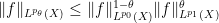
Lemma 9 (Log-convexity of
and
. Then
for all
, and furthermore we have
for all
is defined by
.
In particular, we see that the function
is log-convex whenever the right-hand side is finite (and is in fact log-convex for all
, if one extends the definition of log-convexity to functions that can take the value
). In other words, we can interpolate any two bounds
and
to obtain
for all
Let us give several proofs of this lemma. We will focus on the case 

The first proof is to use Hölder’s inequality

when 

Another (closely related) proof proceeds by using the log-convexity inequality

for all 


A third approach is more in the spirit of the real interpolation method, avoiding the use of convexity arguments. As in the second proof, we can reduce to the normalised case 


and similarly

and so by the quasi-triangle inequality (or triangle inequality, when 
for some constant 

This is off by a constant factor by what we want. But one can eliminate this constant by using the tensor power trick. Indeed, if one replaces 


for all 

for every 


Finally, we give a fourth proof in the spirit of the complex interpolation method. By replacing 


Exercise 10 If
Now we consider variants of interpolation in which the “strong” ![{\lambda_f: {\bf R}^+ \rightarrow [0,+\infty]}](https://s0.wp.com/latex.php?latex=%7B%5Clambda_f%3A+%7B%5Cbf+R%7D%5E%2B+%5Crightarrow+%5B0%2C%2B%5Cinfty%5D%7D&bg=ffffff&fg=000000&s=0&c=20201002)
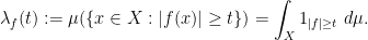
This distribution function is closely connected to the

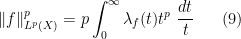
and the Fubini-Tonelli theorem, we obtain the formula
for all 

Exercise 11 Show that we have the relationship
for any measurable
to denote a pair of inequalities of the form
for some constants
depending only on
is non-increasing in
of the distribution function; indeed, for any
is comparable (up to constant factors depending on
norm of the sequence
.

Another relationship between the

for any 
(The 


Chebyshev’s inequality motivates one to define the weak 

thus Chebyshev’s inequality can be expressed succinctly as

It is also natural to adopt the convention that 


and hence

this easily leads to the quasi-triangle inequality

where we use 


Let
Example 12 If
with the usual measure, and
is in weak
for any other
. But the “local” component
of
, and the “global” component
of
.
Exercise 13 For any
and
to be
norm of the sequence
be the space of functions
and to
. Lorentz spaces arise naturally in more refined applications of the real interpolation method, and are useful in certain “endpoint” estimates that fail for Lebesgue spaces, but which can be rescued by using Lorentz spaces instead. However, we will not pursue these applications in detail here.
Exercise 14 Let
(Hint: to prove the second inequality, normalise
, and then manually dispose of the regions of

One can interpolate weak 

for all

and

for all 
As remarked in the previous section, we can improve upon (11); indeed, if we define 


for some 

for some constant 


Exercise 15 Let


Define the strong type diagram of a function 
Exercise 16 Let
such that
for all
for all
. (Hint: first look for the formula that describes
for some
in terms of
is known as the non-increasing rearrangement of
Exercise 17 Let
be a
, and
for some finite
- There exists a constant
for all sets
Furthermore show that the best constants
in the above statements are equivalent up to multiplicative constants depending on
. Conclude that the modified weak
, where
Exercise 18 Let
be an integer. Find a probability space
with
for
such that
for some absolute constant
. (Hint: exploit the logarithmic divergence of the harmonic series
.) Conclude that there exists a probability space
quasi-norm is not equivalent to an actual norm.
Exercise 19 Let
- There exists a constant
with
such that
.
Exercise 20 Let
- There exists a constant
such that
for all
.
- There exists a constant
such that
.
— 3. Interpolation of operators —
We turn at last to the central topic of these notes, which is interpolation of operators 


A typical situation is that of a linear operator 


for all 


The complex interpolation method gives a satisfactory result as long as the exponents allow one to use duality methods, a result known as the Riesz-Thorin theorem:
Theorem 21 (Riesz-Thorin theorem) Let
. Let
be a linear operator obeying the bounds (13), (14) for all
for all
, where
, and
.

Remark 22 When
Proof: If 


By Hölder’s inequality, the bound (13) implies that
for all 


 .
.
for all 


![\displaystyle F(s) := \int_Y (T [ |f|^{(1-s) p_\theta/p_0 + s p_\theta/p_1} \hbox{sgn}(f) ]) [ |g|^{(1-s) q'_\theta/q'_0 + s q'_\theta/q'_1} \hbox{sgn}(g) ]\ d\nu](https://s0.wp.com/latex.php?latex=%5Cdisplaystyle+F%28s%29+%3A%3D+%5Cint_Y+%28T+%5B+%7Cf%7C%5E%7B%281-s%29+p_%5Ctheta%2Fp_0+%2B+s+p_%5Ctheta%2Fp_1%7D+%5Chbox%7Bsgn%7D%28f%29+%5D%29+%5B+%7Cg%7C%5E%7B%281-s%29+q%27_%5Ctheta%2Fq%27_0+%2B+s+q%27_%5Ctheta%2Fq%27_1%7D+%5Chbox%7Bsgn%7D%28g%29+%5D%5C+d%5Cnu&bg=ffffff&fg=000000&s=0&c=20201002)
(with the conventions that 


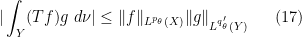
The estimate (17) has currently been established for simple functions 


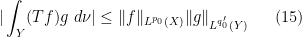
Suppose one has a linear operator 


![{[0,+\infty) \times [0,1]}](https://s0.wp.com/latex.php?latex=%7B%5B0%2C%2B%5Cinfty%29+%5Ctimes+%5B0%2C1%5D%7D&bg=ffffff&fg=000000&s=0&c=20201002)

![{[0,1] \times [0,+\infty)}](https://s0.wp.com/latex.php?latex=%7B%5B0%2C1%5D+%5Ctimes+%5B0%2C%2B%5Cinfty%29%7D&bg=ffffff&fg=000000&s=0&c=20201002)

Exercise 23 If
with the usual measure, show that the strong type diagram of the identity operator is the triangle
. If instead
with the usual counting measure, show that the strong type diagram of the identity operator is the triangle
. What is the strong type diagram of the identity when
with the usual measure?
Exercise 24 Let
) be a linear operator from simple functions of finite measure support on
are formally adjoint if we have
for all simple functions
of finite measure support on
respectively. If
, show that
. Thus, taking formal adjoints reflects the strong type diagram around the line of duality
, at least inside the Banach space region
.
Remark 25 There is a powerful extension of the Riesz-Thorin theorem known as the Stein interpolation theorem, in which the single operator
for
that vary holomorphically in
is a holomorphic function of
of finite measure. Roughly speaking, the Stein interpolation theorem asserts that if
is of strong type
for
with a bound growing at most exponentially in
will be of strong type
Now we turn to the real interpolation method. Instead of linear operators, it is now convenient to consider sublinear operators ![{[0,+\infty]}](https://s0.wp.com/latex.php?latex=%7B%5B0%2C%2B%5Cinfty%5D%7D&bg=ffffff&fg=000000&s=0&c=20201002)
and the pointwise bounds

and
for all 
Every linear operator is sublinear; also, the absolute value 


The basic theory of sublinear operators is similar to that of linear operators in some respects. For instance, continuity is still equivalent to boundedness:
Exercise 26 Let
. Assume that either
- There exists a constant
such that
for all simple functions
Show that the extension mentioned above is unique. Finally, show that the same equivalences hold if
throughout.
We say that 
We now give the real interpolation counterpart of the Riesz-Thorin theorem, namely the Marcinkeiwicz interpolation theorem:
Theorem 27 (Marcinkiewicz interpolation theorem) Let
and
, and
for
. Let
Remark 28 Of course, the same claim applies to linear operators
. One can also extend the argument to quasilinear operators, in which the pointwise bound
is replaced by
for some constant
can be replaced by the variant condition
(see Exercise 31, Exercise 33), but cannot be eliminated entirely: see Exercise 32. The precise hypotheses required on
are rather technical and I recommend that they be ignored on a first reading.
Proof: For notational reasons it is convenient to take 
By hypothesis, there exist constants


for all simple functions 

By homogeneity we can normalise 
Actually, it will be more slightly convenient to work with the dyadic version of the above estimate, namely

see Exercise 11. The hypothesis
The basic idea is then to get enough control on the numbers 

When 


where 


where 

From sublinearity we have the pointwise estimate
which implies that
whenever 

From (18), (19), we have two bounds for the quantity 

and

From construction of

and similarly for

for

It is convenient to introduce the quantities 

and our task is to show that

Since 

 .
.We can simplify this expression a bit by collecting terms and making some substitutions. The points 
for some 


Note that 


Remark 29 A closer inspection of the proof (or a rescaling argument to reduce to the normalised case
for all simple functions
. Thus the conclusion here is weaker by a multiplicative constant from that in the Riesz-Thorin theorem, but the hypotheses are weaker too (weak-type instead of strong-type). Indeed, we see that the constant
must blow up as

The power of the Marcinkiewicz interpolation theorem, as compared to the Riesz-Thorin theorem, is that it allows one to weaken the hypotheses on

for all sets 
Exercise 30 Show that the Marcinkiewicz interpolation theorem continues to hold if the weak-type hypotheses are replaced by restricted weak-type hypothesis. (Hint: where were the weak-type hypotheses used in the proof?)
We thus see that the strong-type diagram of 
Exercise 31 Suppose that
.
Exercise 32 For any
be the natural numbers
with the weighted counting measure
, thus each point
. Show that if
, then the identity operator from
is of weak-type
and
. Conclude that the hypotheses
Exercise 33 Suppose we are in the situation of the Marcinkiewicz interpolation theorem, with the hypotheses
there exists a
for all simple functions
were defined in Exercise 13. (Hint: repeat the proof of the Marcinkiewicz interpolation theorem, but partition the sum
into regions of the form
for integer
. Obtain a bound for each summand which decreases geometrically as
.) Conclude that the hypotheses

Exercise 34 For
, let
be
be a linear operator from simple functions of finite measure support on
to measurable functions on
(modulo almost everywhere equivalence, as always). Let
,
be the product spaces (with product
of product sets of sets
,
of finite measure, such that
for a.e.
; we refer to
and
and write
. Show that if
are of strong-type
with operator norms
respectively, then
, thus
(Hint: for the lower bound, show that
for all simple functions
. For the upper bound, express
as the composition of two other operators
and
for some identity operators
, and establish operator norm bounds on these two operators separately.) Use this and the tensor power trick to deduce the Riesz-Thorin theorem (in the special case when
for


Exercise 35 (Hölder’s inequality for Lorentz spaces) Let
and
for some
. Show that
, where
and
, with the estimate
for some constant
. (This estimate is due to O’Neil.)

Remark 36 Just as interpolation of functions can be clarified by using step functions
as a test case, it is instructive to use rank one operators such as
where
are finite measure sets, as test cases for the real and complex interpolation methods. (After understanding the rank one case, I then recommend looking at the rank two case, e.g.
, where
could be very different in size from
.)
— 4. Some examples of interpolation —
Now we apply the interpolation theorems to some classes of operators. An important such class is given by the integral operators

from functions 
which is well-defined (though it may be infinite).
The following useful lemma gives us strong-type bounds on 

Lemma 37 (Schur’s test) Let
for almost every
, and
for almost every
, where
and
well-defined for all
Here we adopt the convention that
and
, thus
and
.


Proof: The hypothesis 
for all 

Similarly, Hölder’s inequality tells us that for 

Applying the Riesz-Thorin theorem we conclude that

for all simple functions 
for all simple functions
Example 38 Let
be a matrix such that the sum of the magnitudes of the entries in every row and column is at most
, i.e.
for all
and
for all
. Then one has the bound
for all vectors
and all
A useful special case arises when
.

Exercise 39 Establish Schur’s test by more direct means, taking advantage of the duality relationship
for
for
. (You may wish to first work out Example 38, say with

A useful corollary of Schur’s test is Young’s convolution inequality for the convolution 


provided of course that the integrand is absolutely convergent.
Exercise 40 (Young’s inequality) Let
be such that
. Show that if
and
, then
, and furthermore that
(Hint: Apply Schur’s test to the kernel
.)

Remark 41 There is nothing special about
here; one could in fact use any locally compact group
with a bi-invariant Haar measure. On the other hand, if one specialises to
where
, a result of Beckner; the constant here is best possible, as can be seen by testing the inequality in the case when

Exercise 42 Let
. Young’s inequality tells us that
. Refine this further by showing that
, i.e.
, then use a limiting argument.)
We now give a variant of Schur’s test that allows for weak estimates.
Lemma 43 (Weak-type Schur’s test) Let
for almost every
for almost every
and
are now excluded). Then for every
Here we again adopt the convention that

Proof: From Exercise 17 we see that

for any measurable 


for any

thus 
whenever 


This leads to a weak-type version of Young’s inequality:
Exercise 44 (Weak-type Young’s inequality) Let
be such that
, then
for some constant
.

Exercise 45 Refine the previous exercise by replacing
throughout.
Recall that the function 


Corollary 46 (Hardy-Littlewood-Sobolev fractional integration inequality) Let
and
be such that
. If
, defined as
is well-defined almost everywhere and lies in
for some constant
.

This inequality is of importance in the theory of Sobolev spaces, which we will discuss in a subsequent lecture.
Exercise 47 Show that Corollary 46 can fail at the endpoints
, or
.
Update, Apr 6: another exercise added; note renumbering.
Update, Apr 8: some formatting errors fixed.
Update, Sep 14: definition of sublinearity fixed.

137 comments
Comments feed for this article
4 April, 2010 at 8:22 am
pavel zorin
Dear Prof. Tao,
some errata for your proof of the Marcinkiewicz interpolation theorem:
In equation (22), there should be no summation over m.
In the last equation (“simplify the left-hand side of (22) to…”), the summation goes over n instead of m, and the exponent of is
is  , not
, not  .
.
This affects the choice of the c’s, i.e. with
with  would do. The normalization sequence satisfies $d(n) = O(1)$ automatically given
  .
.
I also wonder whether, at the end of the proof of the Riesz-Thorin theorem, the decomposition of f into a bounded and a finitely supported function could be omitted in case (when the sum of the norms of the components is greater then the norm of f itself). It does provide continuity of
  (with norm 2), so that the conclusion follows because it actually has norm 1 on a dense subspace (of simple functions), but can one do without it?
best regards, pavel
4 April, 2010 at 9:21 am
Terence Tao
Thanks for the correction!
One can try to extend the main argument directly to general functions rather than just to simple functions with finite measure support; from a conceptual viewpoint this is more natural, but from a technical viewpoint it basically requires one to establish the continuity of
  to
to  beforehand to justify various formal operations, which is inconvenient as this is part of what one is trying to prove in the first place.
7 April, 2010 at 2:13 pm
pavel zorin
Dear Prof. Tao,
I am experiencing slight difficulties with Exercise 21 (Marcinkiewicz theorem, Lorentz space version).
Doing the same calculations as in the given proof of the special case, I obtain (this time with and
and  ), as a sufficient condition the existence of summable (over m) c’s such that
 .
.
Now, assuming the easiest case , the exponent of
  is less than 1 for one of the i's (unless
  ). Even then, I could not think of an approach to finding c's that uses all the information: whatever I came up with looked like it would work without any assumptions on a's and was therefore false. Could you give some further indications?
kind regards, pavel
7 April, 2010 at 3:02 pm
Terence Tao
Ah, yes, this is a little delicate, in part because the decomposition of f used here is actually not the optimal one for this problem – it decomposes the height of the function dyadically (vertical dyadic decomposition), when in fact it is the width
  that ought to be dyadically decomposed (horizontal dyadic decomposition). One can still recover from this point by decomposing the sequence
  into dyadic pieces, but this is quite messy.
Another approach is to use frequency envelopes. Pick a small and replace
  by the slightly larger envelope
  . The point of doing so is that the
  obey a Lipschitz property
  but are still summable in
  . One then chooses
  to be adapted to the crossover point between the two quantities in the
  (modifying the
  term by some multiple of
  ); as long as the Lipschitz parameter
  is small enough, one will still be able to close the argument.
I may elaborate on the frequency envelope approach in a subsequent blog post.
14 April, 2011 at 4:28 pm
Wenying Gan
Dear Prof. Tao:
I think there is a typo in $Ex 8$. There should be a index 1/p for log(1+|X|). Or the result we need to prove is incorrect. Thanks in advance.
Best
Wenying Gan
[Corrected, thanks – T.]
4 November, 2012 at 6:13 pm
Gandhi Viswanathan
Dear Professor Tao,
The “Control Level Sets” tricki page you cite earlier also lacks the (1/p) index mentioned in this comment about Ex 8. Can we assume the same correction is needed in the tricki ?
4 November, 2012 at 6:21 pm
Terence Tao
Yes; I edited the tricki page accordingly.
4 November, 2012 at 6:49 pm
Gandhi Viswanathan
Thanks!
3 May, 2011 at 6:22 pm
Stein’s interpolation theorem « What’s new
[…] where are functions depending on in a suitably analytic manner, for instance taking for some test function , and similarly for . If are chosen properly, will depend analytically on as well, and the two hypotheses (1), (2) give bounds on and for respectively. The Lindelöf theorem then gives bounds on intermediate values of , such as ; and the Riesz-Thorin theorem can then be deduced by a duality argument. (This is covered in many graduate real analysis texts; I myself covered it here.) […]
4 April, 2012 at 12:50 am
X
Dear Prof. Tao, is very small, then if
  , then the bound goes to
  . So I think the theorem doesn’t cover directly the case where the bound is, for example,
  .
.
There is one thing unclear for me In your statement of Lindelof’s Theorem. Suppose
Could you please help explain a bit?
Thank you!
X
4 April, 2012 at 7:14 am
Terence Tao
The factor will damp out the growth as
  .
.
31 October, 2012 at 9:10 am
Gandhi Viswanathan
Dear Professor Tao, I noticed that the quantity defined via
  in the complex analysis (4th) proof of Lemma 2 above is identical to the quantity
  defined below Lemma 2 in the 2nd proof (via Jensen’s inequality).
4 March, 2013 at 3:13 pm
Lior Silberman
In Remark 2, should be
  .
.
[Corrected, thanks – T.]
23 September, 2013 at 10:54 am
Anonymous
Dear Professor Tao,
I was wandering if for $p1$ such that $\frac{1}{p}+\frac{1}{q}=2$ one has a young type inequality for the convolution. That is $||f*g||_{1}\leq C||f||_{p} ||g||_{q}$
Thanks!
27 April, 2014 at 12:34 pm
Fan
For remark 8, is it necessary that the Haar measure is “bi”-invariant? Is the commutativity of the convolution implicitly used anywhere?
27 April, 2014 at 2:02 pm
Terence Tao
The bi-invariance of Haar measure is needed in order to ensure the map is measure-preserving, otherwise one has to be very careful how to define convolution, as various definitions of convolution that are equivalent in the bi-invariant setting may now cease to be equivalent.
27 April, 2014 at 2:20 pm
Fan
Thanks.
5 May, 2014 at 6:49 am
urbano
Dear Professor Tao, ?
?
is it also possible to show that
4 February, 2015 at 3:40 am
Felix V.
Dear Prof. Tao, thanks for the nice post.
One small comment: In equation (7) in the statement of Lindelöf’s theorem, I believe you want to put |t| instead of t in the exponent of the right hand side. Otherwise, the theorem still holds true, but the statement is needlessly weak.
Best regards, Felix V.
[Corrected, thanks – T.]
19 February, 2015 at 4:36 am
Felix V.
Dear Prof. Tao,
I think I found a problem in Exercise 17: For sublinear operators,
 .
.
it seems that “boundedness” in the sense of
for all step functions does not(!) imply that T can be extended
continuously to all of
My counterexample is the following: Define for simple functions

 can be regarded as an
  -space on a singleton
 ,
,


Here,
set. For simple functions, Tf is indeed well-defined with
which implies
and
so that T is indeed sublinear and “bounded”.
But T itself is not continuous (and thus admits no continuous extension) -norm: If we take
 ![f:=\chi_{\left[0,1\right]}](https://s0.wp.com/latex.php?latex=f%3A%3D%5Cchi_%7B%5Cleft%5B0%2C1%5Cright%5D%7D&bg=ffffff&fg=545454&s=0&c=20201002)
![f_{n}:=\chi_{\left[0,1\right]}+\frac{1}{n}\chi_{\left[10+n,10+2n\right]}](https://s0.wp.com/latex.php?latex=f_%7Bn%7D%3A%3D%5Cchi_%7B%5Cleft%5B0%2C1%5Cright%5D%7D%2B%5Cfrac%7B1%7D%7Bn%7D%5Cchi_%7B%5Cleft%5B10%2Bn%2C10%2B2n%5Cright%5D%7D&bg=ffffff&fg=545454&s=0&c=20201002) ,
, , but $Tf=e^{i\pi}\left\Vert f\right\Vert _{2}=-1$ and
 .
.
with respect to the
and
then
for
Best regards, Felix V.
19 February, 2015 at 4:40 am
Felix V.
Oh, I just noted that you require to have values in
 ![[0,\infty]](https://s0.wp.com/latex.php?latex=%5B0%2C%5Cinfty%5D&bg=ffffff&fg=545454&s=0&c=20201002) . But you also claim that every linear operator is sublinear, which certainly does not hold if we require values in
. But you also claim that every linear operator is sublinear, which certainly does not hold if we require values in ![[0,\infty]](https://s0.wp.com/latex.php?latex=%5B0%2C%5Cinfty%5D&bg=ffffff&fg=545454&s=0&c=20201002) .
.
19 February, 2015 at 9:56 am
Terence Tao
Sorry, there was an additional hypothesis in the definition of sublinearity (namely that ) that was not corrected in the post (though it was noted in the errata for the published version of these notes).
25 November, 2015 at 10:07 am
Anon
Typo? In Riesz-Thorin Theorem missing parantheses around 1-\theta?
[Corrected, thanks – T.]
2 December, 2015 at 12:06 am
Anonymous
Dear Prof. Tao,
I guess that in Lemma 9, $p$ and $L^p(X)$ should be replaced by $p_\theta$ and $L^{p_\theta}(X)$, resp.
[Actually, I prefer to leave the qualitative portion of the lemma (which I presume is the part you are referring to) in terms of a parameter instead of a
  parameter, as the latter is only useful for the quantitative estimate. -T.]
11 December, 2015 at 5:19 pm
Anonymous
About Exercise 16,
I think Exercise 16 should be corrected a little bit. If substitute t with 0 and f*(0) respectively, we might have the measure of X is infinite and ||f||_{inf}<= f*(0)
http://math.stackexchange.com/questions/257365/questions-related-to-distribution-function-and-its-inverse
In this site, altering some of the definitions and conditions makes things going well.
It would be appreciated if you check.
[The case should not have been present and is now deleted – T.]
12 December, 2015 at 3:55 am
Anonymous
Dear Prof. Tao,
In Exercise 17, is p` is the dual exponent of p?
[Corrected, thanks – T.]
26 December, 2015 at 4:52 pm
Jiwoong Jang
Dear Prof. Tao,
In the exercise about the marcinkiewicz theorem on the Lorentz spaces, I see your point that adopting the frequency envelope b_m of a_m works, but only in the particular case of $r<=q_\theta$. If r is large, I still do not know how to eliminate the r portion of the exponent of b_m.
Could you give me a direction to go? Or, Is it enough to prove all the things? I`m now considering the quasi-metric structure of $l^{q_\theta/r}(\mathbb{Z})$.
Best
Jang
1 June, 2016 at 6:58 pm
Anonymous
… from the calculus identity
and the Fubini-Tonelli theorem, we obtain the formula…
Some typo here? The left hand side is a function in while the right hand side is a number?
[The on the RHS should be
  , now fixed – T.]
27 June, 2016 at 9:08 am
Benson
Dear Prof,
Is there any work done on application of any of the interpolation theorems to signal and image processing . I will like to know.
11 October, 2016 at 6:58 am
Lecture 9. Diffusion semigroups in L^p | Research and Lecture notes
[…] proof of the theorem can be found in this post by […]
3 December, 2016 at 5:10 am
VMT
Hi Professor, with
with  .
. a sufficiently small multiple of
  , where
  .
.
I have some little corrections to your instructive proof of Marcinkiewicz interpolation:
in (22) there should be only the sum over n.
In the last display of the proof, m should be replaced with n and
I guess one should then take
Finally, there are three references to (16), (19) which should be replaced with (18), (19).
[Corrected, thanks – T.]
23 January, 2017 at 3:41 pm
Anonymous
(1) In Section 3, what is the definition of ? Is it the same or different from the “direct sum”?
[No: see https://en.wikipedia.org/wiki/Minkowski_addition – T.]
(2) In Stein and Weiss’s Introduction to Fourier Analysis on Enclidean Spaces, the linear operator in the Riesz-Thorin Theorem is defined on a set of simple functions of sets of finite measures. Are that version equivalent to the one in this note? Is there any historical reason or theoretical convenience in Stein-Weiss’s version?
[It makes little difference in practice, since a bounded linear operator on a dense subclass of a normed vector space can always be uniquely extended to a bounded linear operator on the full space. -T.]
25 January, 2017 at 4:37 am
Anonymous
In remark 29 (lines 4 and 7), it seems that the constant (with several subscripts) should not contain the subscript
  .
.
Is the best possible constant (as a function of its subscripts) known up to a multiplication by an absolute constant?
[Yes – I believe this is discussed for instance in Bergh and Lofstrom. -T.]
21 February, 2017 at 11:13 am
Anonymous
– Right after (6), would you elaborate what the following remark means?
The geometric series formula tells us that such factors are absolutely summable, and so in practice it is often a useful heuristic to pretend that the cases dominate so strongly that the other cases can be viewed as negligible by comparison.
Do you have an example when one would like to sum the factors ?
?
– “However, one certainly cannot interpolate lower bounds: (i)lower bounds on a log-convex function {\theta \rightarrow A_\theta} at {\theta=0} and {\theta=1} yield no information about the value of, say, {A_{1/2}}. (ii)Similarly, one cannot extrapolate upper bounds on log-convex functions: an upper bound on, say, {A_0} and {A_{1/2}} does not give any information about {A_1}. (However, an upper bound on {A_0} coupled with a lower bound on {A_{1/2}} gives a lower bound on {A_1}; this is the contrapositive of an interpolation statement.)”
I’m a little confused with this remark. For (i), if one looks at the log-convex function (5), then (3) means one can interpolate lower bounds?
25 February, 2017 at 10:30 am
Terence Tao
See for instance the argument deriving (12) from (11) (here we use a continuous variable instead of a discrete one
  , but the principle is the same. See also the proof of Theorem 27.)
The function in (5) is log-convex as well as log-concave, which is why one can interpolate lower bounds for that function. However, most log-concave functions will not be log-convex.
21 February, 2017 at 5:20 pm
Anonymous
In the second proof Lemma 9, one can divide by its
  or
or  norm to achieve one of the normalizations. How can one do it simultaneously for both? Why is the measure
  also allowed to change?
25 February, 2017 at 10:33 am
Terence Tao
If is a measure space, then so is
  for any
  . It is then a simple matter of algebra to find, given any measure space
  and any
  in both
  and
and  of that space, constants
  such that
  . If we know how to prove Lemma 9 in this case, a little further algebra then recovers Lemma 9 in the general case.
23 February, 2017 at 3:03 pm
Anonymous
In the third proof of Lemma 9, typos in the tensor power:
The component x_m should be x_M and the underlying measure space for the tensor power should be X^M
[Corrected, thanks – T.]
25 February, 2017 at 1:37 pm
Anonymous
One more in
we see from many applications of the Fubini-Tonelli theorem that
the left hand side should be
[Corrected, thanks – T.]
5 March, 2017 at 2:52 pm
Anonymous
In the set of your notes (http://www.math.ucla.edu/~tao/247a.1.06f/notes1.pdf) on harmonic analysis, the first sentence of the introduction to the Vinogradov notation is very confusing (page 5):
In (modified) Vinogradov notation, the notation (read:
  is less than or
 ) or
) or  is used synonymously with
  or
or  .
.
comparable to
I think you mean
just as indicated in this post?
[Correction added to 247a page, thanks -T.]
10 March, 2017 at 3:38 pm
Anonymous
In the first proof of Lemma 9, Hölder is used. It is said in your 247a notes 1 that Lemma 9 actually implies Hölder also.
The hint there says that one should consider the convexity of with respect to a measure
  for some constants
  .
.
I don’t understand what this really means. Would you elaborate a little bit more?
[Apply Lemma 9 with replaced by
  and
and  replaced by
  , and for a carefully selected choice of
  . -T]
. -T]
11 March, 2017 at 5:15 pm
Anonymous
1. Suppose one wants to prove the Holder with
with  . Suppose in Lemma 9,
  with
with  . One can then choose any
  with
with  , then let

and
The constants do not need to be unique, right?
2. It is said in the hint that one needs to first reduce to the case of finite measure space and and
and  everywhere non-vanishing simple functions. Why is that so? It seems that one can get the proof by directly manipulate the constants so that one can match the exponents of the two inequalities (Holder and the log-convexity).
[One needs various norms to be finite and non-zero in order to justify some algebraic manipulations, such as raising these norms to a negative power. -T]
17 November, 2017 at 1:11 pm
Anonymous
Why can one replace by
by  in Lemma 9? Isn’t Lemma 9 only true when one replace
  by
by  where
where  is a (nonnegative) constant?
26 November, 2017 at 10:19 am
Terence Tao
Lemma 9 is true for arbitrary non-negative measures , which gives one the (powerful) freedom to multiply
  by arbitrary non-negative weights, not just constants.
17 November, 2017 at 1:38 pm
Anonymous
I attempted what was suggested directly:
which seems not quite true…
26 November, 2017 at 10:30 am
Terence Tao
This is a correct inequality. One now has to select the parameters carefully to obtain the desired conclusion.
20 November, 2017 at 6:45 pm
Anonymous
Suppose one wants to prove Hölder for . Assume the log-convexity for
  . Apply Lemma 9 with
  replaced by
  and
and  replaced by
  . Comparing the exponents, we want

So if we let such that
  and
and
![\displaystyle r'=r,\ \ p'=(1-\theta)p,\ \ q'=\theta q\\ \alpha = \frac{p}{[(1-\theta)p-\theta q]}\\ \beta = \frac{q}{\theta q-(1-\theta)p}\\ \delta = -\beta p'\\ \gamma = -\alpha q'](https://s0.wp.com/latex.php?latex=%5Cdisplaystyle+r%27%3Dr%2C%5C+%5C+p%27%3D%281-%5Ctheta%29p%2C%5C+%5C+q%27%3D%5Ctheta+q%5C%5C+%5Calpha+%3D+%5Cfrac%7Bp%7D%7B%5B%281-%5Ctheta%29p-%5Ctheta+q%5D%7D%5C%5C+%5Cbeta+%3D+%5Cfrac%7Bq%7D%7B%5Ctheta+q-%281-%5Ctheta%29p%7D%5C%5C+%5Cdelta+%3D+-%5Cbeta+p%27%5C%5C+%5Cgamma+%3D+-%5Calpha+q%27+&bg=ffffff&fg=545454&s=0&c=20201002)
then we have the desired result.
Where one needs to first reduce to the case of finite measure space and f and g everywhere non-vanishing simple functions?
26 November, 2017 at 10:31 am
Terence Tao
If some of the exponents are negative, you will have a division by zero problem if one did not prepare in advance by reducing to the case when
  were everywhere non-vanishing.
10 March, 2017 at 4:39 pm
Anonymous
In 247a notes 1 Problem 5.9, it is said that one can differentiate twice with respect to
  to get the log convexity of the
  norm. Why should one use
  instead of
  ?
?
[The function is convex, but the function
  is usually not convex. -T.]
10 March, 2017 at 4:43 pm
Anonymous
As it is mentioned in the notes, this approach is messy. Has anyone performed the calculation ever to show that this is indeed doable? (Lots of terms would appear when calculating the second derivative. Still possible to see that the second derivative is positive?)
13 March, 2017 at 7:32 am
Anonymous
Another version of (7) in Theorem is given in the 247a notes 1:
Are these two versions equivalent? (Since it could be that and a positive constant is missing in front of the "inner" exponential function in (7), I'm not sure about this.)
[Yes, they are equivalent. Note that one has the freedom to reduce if desired, in particular one can assume that
  is positive. -T]
13 March, 2017 at 10:45 am
Anonymous
According to this set of notes
holomorphic functions are defined on open subsets of . What does the function
  being holomorphic on the strip
  (which is closed) mean? (What does one mean that
  is holomorphic on the boundary?)
[It means that the function extends to be holomorphic on some open neighbourhood of the strip. -T]
13 March, 2017 at 11:43 am
Anonymous
In the proof of Theorem 4, would you elaborate why is the function holomorphic and non-zero on
  ?
?
Isn’t it true that one needs to define using the complex logarithm, which is not holomorphic at
  ? Moreover, what branch one needs to use for the function
  ?
?
[One only needs to take logarithms of the positive real constants ; at no point does one need to take logarithms of the complex variable
  . -T]
. -T]
17 March, 2017 at 7:37 am
Anonymous
In the last step of passage to the limit of Theorem 21 (Riesz-Thorin theorem), one decomposes into a bounded function and a function of finite measure support and then approximates each piece by simple functions. How would one put the two approximations together to get the approximation for
  ?
?
18 March, 2017 at 6:37 am
Anonymous
In Lemma 9 and Theorem 21; the exponents are in
 ![[0,\infty]](https://s0.wp.com/latex.php?latex=%5B0%2C%5Cinfty%5D&bg=ffffff&fg=545454&s=0&c=20201002) while the
while the  are in
 ![[1,\infty]](https://s0.wp.com/latex.php?latex=%5B1%2C%5Cinfty%5D&bg=ffffff&fg=545454&s=0&c=20201002) . Can we change the range for
. Can we change the range for  to be also in
 ![[0,\infty]](https://s0.wp.com/latex.php?latex=%5B0%2C%5Cinfty%5D&bg=ffffff&fg=545454&s=0&c=20201002) ? (Or is there a typo so that the
? (Or is there a typo so that the  should also in
 ![[1,\infty]](https://s0.wp.com/latex.php?latex=%5B1%2C%5Cinfty%5D&bg=ffffff&fg=545454&s=0&c=20201002) ?)
?)
18 March, 2017 at 6:43 am
Anonymous
It is said at the beginning of section 3 that “much of the theory here extends to the non- -finite setting.”
Is the -finite assumption implicitly used somewhere in the proof of Theorem 21? (Or is the theorem true in the non-
 -finite setting?)
19 March, 2017 at 6:09 am
Anonymous
In Lemma 9, what norm should one use for the space ?
?
In Theorem 21, what norm should one use for the Minkowski sums and
and  ?
?
22 March, 2017 at 6:05 am
Terence Tao
I don’t believe I using a norm for these spaces anywhere in my text, but the standard norm on the intersection of two normed vector spaces is defined as
  (one can also use the equivalent norm
  ), and the standard norm on the sum
  is
is  .
.
19 March, 2017 at 10:16 am
Anonymous
In the definition of the distribution function, several other books (e.g. Folland) use instead of
  in the formula
In practice of doing analysis (in the case that ), how much difference would this make? For instance, would it affect the proof of Mincinkiewicz interpolation theorem?
6 December, 2017 at 7:10 am
Anonymous
Instead of being right-continuous, one gets being left-continuous here. That’s the only difference I think. In practice, may be not a big deal.
6 December, 2017 at 7:08 am
jack
It is said in Wikipedia (https://en.wikipedia.org/wiki/Lorentz_space) that the Lorentz space norm with
with  is the area of the largest rectangle with sides parallel to the coordinate axes that can be inscribed in the graph.
However, direct calculation shows that the area of any inscribed rectangle is
What goes wrong? Can it be explained by Exercise 13?
6 December, 2017 at 7:15 am
Anonymous
The Lorentz norm of an indicator function can be calculated easily. But when it goes to general functions, even just simple functions, the calculation becomes much more difficult. What is this norm really about?
Maybe its property such as is more important than what it really is?
6 December, 2017 at 12:33 pm
Terence Tao
Yes, the Lorentz space norm of this function is equal to . As it turns out the dyadic Lorentz space norm is also equal to
  . (In general, the two expressions will be comparable, but not identical.) I find the dyadic norm to be a bit more tractable in computations (for instance it is easy to compute for linear combinations of a few indicator functions, particularly if the sets involved are disjoint and the coefficients are lacunary).
16 December, 2017 at 12:32 pm
Anonymous
In Stein-Weiss, the following inequality is used for the proof of (
( and
and  ):
):
How is this inequality done?
[Upper bound the integral, and then use the monotonicity of norms. -T]
16 December, 2017 at 7:54 pm
Anonymous
Using the monotonicity of norms, one has
![\displaystyle \left(\sum_{k=-\infty}^{\infty} [f^*(2^{k-1})]^{q_2}2^{kq_2/p}\right)^{q_1/q_2} \leq \sum_{k=-\infty}^{\infty} [f^*(2^{k-1})]^{q_1}2^{kq_1/p}](https://s0.wp.com/latex.php?latex=%5Cdisplaystyle++%5Cleft%28%5Csum_%7Bk%3D-%5Cinfty%7D%5E%7B%5Cinfty%7D+%5Bf%5E%2A%282%5E%7Bk-1%7D%29%5D%5E%7Bq_2%7D2%5E%7Bkq_2%2Fp%7D%5Cright%29%5E%7Bq_1%2Fq_2%7D+%5Cleq+%5Csum_%7Bk%3D-%5Cinfty%7D%5E%7B%5Cinfty%7D+%5Bf%5E%2A%282%5E%7Bk-1%7D%29%5D%5E%7Bq_1%7D2%5E%7Bkq_1%2Fp%7D+&bg=ffffff&fg=545454&s=0&c=20201002)
 right.
It seems that one cannot get the exponent in
Rewriting the RHS as
![\displaystyle \sum_{k=-\infty}^{\infty} [f^*(2^{k-1})]^{q_1}2^{kq_1/q_2}(2^{kq_1/p-kq_1/q_2})](https://s0.wp.com/latex.php?latex=%5Cdisplaystyle+%5Csum_%7Bk%3D-%5Cinfty%7D%5E%7B%5Cinfty%7D+%5Bf%5E%2A%282%5E%7Bk-1%7D%29%5D%5E%7Bq_1%7D2%5E%7Bkq_1%2Fq_2%7D%282%5E%7Bkq_1%2Fp-kq_1%2Fq_2%7D%29+&bg=ffffff&fg=545454&s=0&c=20201002)
 should one use?
what
17 December, 2017 at 11:54 am
Anonymous
If in Stein-Weiss, is a typo which should be
  , then the first inequality here has already given the conclusion.
27 January, 2018 at 7:24 pm
Prove $L^{p_theta }(X)subset L^{p_0}(X)+L^{p_1}(X),$ where $frac{1}{p_theta }:=frac{1-theta }{p_0}+frac{theta }{p_1}.$ | Questions
[…] 245C, Notes 1: Interpolation of L^p spaces […]
16 April, 2020 at 5:23 pm
Anonymous
Dear Professor Tao. I have a question regarding the weak spaces. Assume that
  , where the sets
  are disjoints, and
  . Is it true that
with a constant independent of ?
?
Thanks in advance.
16 April, 2020 at 7:12 pm
Terence Tao
No. Consider the case when with counting measure and
  ; then the estimate would be claiming that the
  norm is controlled by the
  norm uniformly in
  , which is false.
10 December, 2020 at 12:09 am
Anonymous
In exercise 14, should be
  instead? there is a similar problem here:https://math.stackexchange.com/questions/762622/inequality-of-strong-lp-and-weak-lp-norm-on-a-finite-set-with-counting-mea
[Corrected, thanks – T.]
13 December, 2020 at 5:13 am
Anonymous
Dear Prof.Tao:
How to continuously extend a linear continuous operator on the subspace of $L^\infty$ to $L^\infty$?
Given any subspace $S$ of $L^\infty$, and $T$ is linear continuous operator on $S$ into some Banach space $B$, is there any general method to extend from $S$ to $L^\infty$ in linear continuous manner?
In this post, it is said that we can maybe non-uniquely extend from the space of simple measurable with finite measure support to $L^\infty$ in a linear continuous manner, how to do this, any hint? I am stuck in this problem, thanks in advance.
13 December, 2020 at 10:32 am
Terence Tao
Both existence and uniqueness are problematic in general. If one of the spaces involves a finite measure then it becomes a complete Banach lattice and the usual proof of Hahn-Banach goes through to give existence of an extension, and sigma-finite measures might still be OK, but I think general measures are not. (There is a theorem of Kelley that says that a Hahn-Banach type extension theorem for a Banach space target
  is possible if and only if
  is isomorphic to the space of continuous functions on a Stonean space, which when applied to
  using Gelfand duality I think comes down to requiring the underlying measure algebra to be complete, which is true when the measure is finite or sigma-finite but I believe there are counterexamples in general.)
13 December, 2020 at 5:59 pm
Anonymous
Is it possible to extend the interpolation theorem with restricted weak-type bounds for operators defined on mixed L^p(L^q) spaces?
13 December, 2020 at 8:32 pm
Terence Tao
Partially, but the more detailed answer is rather complicated; see for instance this paper of Fernandez.
21 July, 2021 at 3:30 am
Gerd Wachsmuth
In Exercise 34, I think one needs for the estimate of
  , see also https://mathoverflow.net/questions/336970/the-norm-of-tensor-product-operator-on-lp-spaces.
Otherwise, it would be possible to deduce the Riesz-Thorin interpolation theorem in the real case with constant $1$ only under the requirement $p_\theta \le q_\theta$ via Marcinkiewicz (or without any requirement via the complex Riesz-Thorin theorem). This, however, is not true, see, e.g., https://link.springer.com/article/10.1007/s000130050241.
[Corrected, thanks – T.]
7 June, 2022 at 11:30 pm
Anonymous
Dear Prof. Tao,
Is it possible to prove the continuous embeddings of L^\infty(L^2)\capL^2(H^1) in L^{4,1}(H^{1/2}) ?
11 June, 2022 at 3:32 pm
Terence Tao
No, there is no such embedding. Consider a function of the form , where
  is a function of frequency
  normalised in
  (so that its
  norm is like
  and its
  norm is like
  ) and the
  are disjoint time intervals of length
  . Then one can check that this function is bounded in
  and
and  but not
  . (More generally, one should experiment with various combinations of rescaled and translated bump functions in order to gain intuition as to whether a given interpolation inequality might be true.)
8 July, 2022 at 2:59 am
Anonymous
Dear prof. Tao,
I read the Riesz Thorin interpolation for vector valued.(For explanation, if i want to get l2 sum of Lp norm, Enough to check sup of L2 and l1 sum of Lq norm) But, Vector valued version RT interpolation that I read has the assumption that the operator T is a linear operator. In the proof, Linearity is needed, when proceeding approximation argument. is it possible to use Vector valued Risez thorin Interpolation theorem for sublinear case?(not marcinkiewicz interpolation for vector valued. It does not interpolate the norm of valued) Would you recommend the refer for this sub linear version of proof?
12 July, 2022 at 2:31 pm
Anonymous
No. Riesz Thorin interpolation only works for linear operators, while Marcinkiewicz interpolation also works for sublinear operators.
12 July, 2022 at 4:58 pm
Anonymous
Thanks for replying!
In page 464 of Harmonic Analysis: Real-Variable Methods, Orthogonality, and Oscillatory Integrals by Stein, I read the middle part of this page using interpolation for sublinear operator. Would you please tell me the interpolation statement they use?
At first, I think, this is the interpolation which is in page 399 problem 5.5.2 of Classical Fourier Analysis by L.Grafakos.
But in here, we need the linearity assumption. You may recommend a reference paper or book for this interpolation.
22 July, 2022 at 4:48 pm
Anonymous
Stein’s book refers to Lorentz spaces interpolation of mixed norms. Dr. Tao mentioned a paper by Fernandez in one of the comments, and the URL is:
Click to access 81999059.pdf
22 July, 2022 at 4:51 pm
Anonymous
Proposition 9.1 on page 143.