
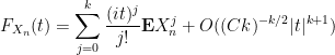
Consider the sum 


then 


In the previous set of notes, we were able to establish various tail bounds on

and if the original distribution 

for some absolute constants 
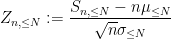
Now we look at the distribution of
Theorem 1 (Central limit theorem) Let
,
.
Exercise 2 Show that
of
, the quantities
and
are almost independent of each other, since the bulk of the sum
is determined by those
with
. Now make this intuition precise.)
Exercise 3 Use Stirling’s formula from Notes 0a to verify the central limit theorem in the case when
and
Exercise 4 Use Exercise 9 from Notes 1 to verify the central limit theorem in the case when
Note we are only discussing the case of real iid random variables. The case of complex random variables (or more generally, vector-valued random variables) is a little bit more complicated, and will be discussed later in this post.
The central limit theorem (and its variants, which we discuss below) are extremely useful tools in random matrix theory, in particular through the control they give on random walks (which arise naturally from linear functionals of random matrices). But the central limit theorem can also be viewed as a “commutative” analogue of various spectral results in random matrix theory (in particular, we shall see in later lectures that the Wigner semicircle law can be viewed in some sense as a “noncommutative” or “free” version of the central limit theorem). Because of this, the techniques used to prove the central limit theorem can often be adapted to be useful in random matrix theory. Because of this, we shall use these notes to dwell on several different proofs of the central limit theorem, as this provides a convenient way to showcase some of the basic methods that we will encounter again (in a more sophisticated form) when dealing with random matrices.
— 1. Reductions —
We first record some simple reductions one can make regarding the proof of the central limit theorem. Firstly, we observe scale invariance: if the central limit theorem holds for one random variable 


The other reduction we can make is truncation: to prove the central limit theorem for arbitrary random variables
Exercise 5 (Linearity of convergence) Let
be a finite-dimensional real or complex vector space,
be sequences of
be another pair of
be scalars converging to
respectively.
- If
converges in distribution to
, and at least one of
converges in distribution to
.
- If
.
- If
.
Show that the first part of the exercise can fail if
Now suppose that we have established the central limit theorem for bounded random variables, and want to extend to the unbounded case. Let 

Let 


converges in distribution to 

For such a sequence, we see from dominated convergence that 


converges in distribution to
Meanwhile, from dominated convergence again, 
converges in distribution to 
Remark 6 The truncation reduction is not needed for some proofs of the central limit theorem (notably the Fourier-analytic proof), but is very convenient for some of the other proofs that we will give here, and will also be used at several places in later notes.
By applying the scaling reduction after the truncation reduction, we observe that to prove the central limit theorem, it suffices to do so for random variables
— 2. The Fourier method —
Let us now give the standard Fourier-analytic proof of the central limit theorem. Given any real random variable 
Equivalently, 

Example 7 The signed Bernoulli distribution has characteristic function
.
Exercise 8 Show that the normal distribution
has characteristic function
.
More generally, for a random variable 

where 


(or equivalently, by identifying 
More generally, one can define the characteristic function on any finite dimensional real or complex vector space 
The characteristic function is clearly bounded in magnitude by 
Exercise 9 (Riemann-Lebesgue lemma) Show that if
as
. Show that the claim can fail when the absolute continuity hypothesis is dropped.
Exercise 10 Show that the characteristic function
Let 
which thus interprets the characteristic function of a real random variable
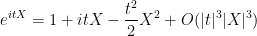
Exercise 11 (Taylor expansion of characteristic function) Let
moment for some
. Show that
times continuously differentiable, and one has the partial Taylor expansion
where
is a quantity that goes to zero as
, times
. In particular, we have
for all
.

Exercise 12 Establish (7) in the case that
Note that the characteristic function depends only on the distribution of 


Theorem 13 (Lévy continuity theorem, special case) Let
- (i)
converges pointwise to
- (ii)
Proof: Without loss of generality we may take 
The implication of (i) from (ii) is immediate from (6) and the definition of convergence in distribution (see Definition 10 of Notes 0), since the function 
Now suppose that (i) holds, and we wish to show that (ii) holds. By Exercise 23(iv) of Notes 0, it suffices to show that

whenever 

where

is a Schwartz function, and is in particular absolutely integrable (see e.g. these lecture notes of mine). From the Fubini-Tonelli theorem, we thus have

and similarly for

Remark 14 Setting
for all
Exercise 15 (Lévy’s continuity theorem, full version) Let
. Show that the following are equivalent:
- (i)
- (ii)
- (iii)
- (iv)
Hint: To get from (ii) to the other conclusions, use Prokhorov’s theorem and Theorem 13. To get back to (ii) from (i), use (8) for a suitable Schwartz function
Remark 16 Lévy’s continuity theorem is very similar in spirit to Weyl’s criterion in equidistribution theory.
Exercise 17 (Esséen concentration inequality) Let
,
, show that
for some constant
depending only on
and
. (Hint: Use (8) for a suitable Schwartz function
.

In Fourier analysis, we learn that the Fourier transform is a particularly well-suited tool for studying convolutions. The probability theory analogue of this fact is that characteristic functions are a particularly well-suited tool for studying sums of independent random variables. More precisely, we have
Exercise 18 (Fourier identities) Let
for all
. Also, for any scalar
, one has
and more generally, for any linear transformation
, one has


Remark 19 Note that this identity (10), combined with Exercise 8 and Remark 14, gives a quick alternate proof of Exercise 9 from Notes 1.
In particular, in the normalised setting (4), we have the simple relationship

that describes the characteristic function of
We now have enough machinery to give a quick proof of the central limit theorem:
Proof: (Proof of Theorem 1) We may normalise
for sufficiently small

for sufficiently small
as 
Exercise 20 (Vector-valued central limit theorem) Let
be a random variable taking values in
to be the
matrix
whose
entry is the covariance
.
- Show that the covariance matrix is positive semi-definite real symmetric.
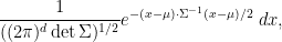
- Conversely, given any positive definite real symmetric
, show that the normal distribution
, given by the absolutely continuous measure
has mean
, and has a characteristic function given by
How would one define the normal distribution
- If
is the sum of
, show that
converges in distribution to
.
Exercise 21 (Complex central limit theorem) Let
, whose real and imaginary parts have variance
and covariance
.
Exercise 22 (Lindeberg central limit theorem) Let
be a sequence of independent (but not necessarily identically distributed) real random variables, normalised to have mean zero and variance one. Assume the (strong) Lindeberg condition
where
is the truncation of
to large values. Show that as
converges in distribution to

A more sophisticated version of the Fourier-analytic method gives a more quantitative form of the central limit theorem, namely the Berry-Esséen theorem.
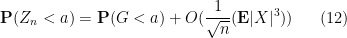
Theorem 23 (Berry-Esséen theorem) Let
, where
are iid copies of
uniformly for all
, where
, and the implied constant is absolute.
Proof: (Optional) Write 

for all 

Let 

![{[-c,c]}](https://s0.wp.com/latex.php?latex=%7B%5B-c%2Cc%5D%7D&bg=ffffff&fg=000000&s=0&c=20201002)

![{1_{(-\infty,0]}}](https://s0.wp.com/latex.php?latex=%7B1_%7B%28-%5Cinfty%2C0%5D%7D%7D&bg=ffffff&fg=000000&s=0&c=20201002)
![\displaystyle \varphi(x) := \int_{\bf R} 1_{(-\infty,0]}(x - \varepsilon y) \eta(y)\ dy.](https://s0.wp.com/latex.php?latex=%5Cdisplaystyle+%5Cvarphi%28x%29+%3A%3D+%5Cint_%7B%5Cbf+R%7D+1_%7B%28-%5Cinfty%2C0%5D%7D%28x+-+%5Cvarepsilon+y%29+%5Ceta%28y%29%5C+dy.&bg=ffffff&fg=000000&s=0&c=20201002)
Observe that
We claim that it suffices to show that

for every 

thus our task is to show that 
Let 


and thus by (13)


Meanwhile, from (14) and an integration by parts we see that

From the bounded density of 

Putting all this together, we see that

A similar argument gives a lower bound

and so

Taking suprema over

If 


It remains to establish (13). Applying (8), it suffices to show that

Now we estimate each of the various expressions. Standard Fourier-analytic computations show that
![\displaystyle \hat \varphi(t) = \hat 1_{(-\infty,a]}(t) \hat \eta(\varepsilon t)](https://s0.wp.com/latex.php?latex=%5Cdisplaystyle+%5Chat+%5Cvarphi%28t%29+%3D+%5Chat+1_%7B%28-%5Cinfty%2Ca%5D%7D%28t%29+%5Chat+%5Ceta%28%5Cvarepsilon+t%29&bg=ffffff&fg=000000&s=0&c=20201002)
and that
![\displaystyle \hat 1_{(-\infty,a]}(t) = O( \frac{1}{1+|t|} ).](https://s0.wp.com/latex.php?latex=%5Cdisplaystyle+%5Chat+1_%7B%28-%5Cinfty%2Ca%5D%7D%28t%29+%3D+O%28+%5Cfrac%7B1%7D%7B1%2B%7Ct%7C%7D+%29.&bg=ffffff&fg=000000&s=0&c=20201002)
Since 

From Taylor expansion we have
for any

and in particular

if 

if 

(say) if
Exercise 24 Show that the error terms here are sharp (up to constants) when
— 3. The moment method —
The above Fourier-analytic proof of the central limit theorem is one of the quickest (and slickest) proofs available for this theorem, and is accordingly the “standard” proof given in probability textbooks. However, it relies quite heavily on the Fourier-analytic identities in Exercise 18, which in turn are extremely dependent on both the commutative nature of the situation (as it uses the identity 

The most elementary (but still remarkably effective) method available in this regard is the moment method, which we have already used in the previous notes, which seeks to understand the distribution of a random variable 
We first need an analogue of the Lévy continuity theorem. Here we encounter a technical issue: whereas the Fourier phases 

Theorem 25 (Moment continuity theorem) Let
- (i) For every
,
converges pointwise to
.
- (ii)
Proof: We first show how (ii) implies (i). Let 
![{[-1,1]}](https://s0.wp.com/latex.php?latex=%7B%5B-1%2C1%5D%7D&bg=ffffff&fg=000000&s=0&c=20201002)
![{[-2,2]}](https://s0.wp.com/latex.php?latex=%7B%5B-2%2C2%5D%7D&bg=ffffff&fg=000000&s=0&c=20201002)


Conversely, suppose (i) is true. From the uniform subgaussian hypothesis, the 


uniformly in

Then letting 


Remark 26 One corollary of Theorem 25 is that the distribution of a subgaussian random variable is uniquely determined by its moments (actually, this could already be deduced from Exercise 12 and Remark 14). The situation can fail for distributions with slower tails, for much the same reason that a smooth function is not determined by its derivatives at one point if that function is not analytic.
The Fourier inversion formula provides an easy way to recover the distribution from the characteristic function. Recovering a distribution from its moments is more difficult, and sometimes requires tools such as analytic continuation; this problem is known as the inverse moment problem and will not be discussed here.
To prove the central limit theorem, we know from the truncation method that we may assume without loss of generality that

for all
The moments 
Exercise 27 Let
when
So now we need to compute 
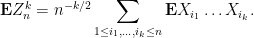
To understand this expression, let us first look at some small values of
- For
, this expression is trivially
- For
, this expression is trivially
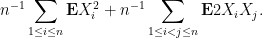
- For
, we can split this expression into the diagonal and off-diagonal components:
Each summand in the first sum is
have mean zero and are independent. So the second moment
is
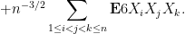
- For
, we have a similar expansion
The summands in the latter two sums vanish because of the (joint) independence and mean zero hypotheses. The summands in the first sum need not vanish, but are
, which is asymptotically negligible, so the third moment
goes to
- For
, the expansion becomes quite complicated:
Again, most terms vanish, except for the first sum, which is
and is asymptotically negligible, and the sum
, which by the independence and unit variance assumptions works out to
. Thus the fourth moment
goes to
(as it should).


Now we tackle the general case. Ordering the indices 


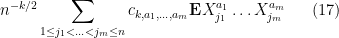
where 

The total number of such terms depends only on 
As we already saw from the small 


On the other hand, the total number of summands in (17) is clearly at most 


and the main term is happily equal to the moment
— 4. The Lindeberg swapping trick —
The moment method proof of the central limit theorem that we just gave consisted of four steps:
- (Truncation and normalisation step) A reduction to the case when
- (Inverse moment step) A reduction to a computation of asymptotic moments
.
- (Analysis step) Showing that most terms in the expansion of this asymptotic moment were zero, or went to zero as
- (Algebra step) Using enumerative combinatorics to compute the remaining terms in the expansion.
In this particular case, the enumerative combinatorics was very classical and easy – it was basically asking for the number of ways one can place 

However, when we apply the moment method to more advanced problems, the enumerative combinatorics can become more non-trivial, requiring a fair amount of combinatorial and algebraic computation. The algebraic miracle that occurs at the end of the argument can then seem like a very fortunate but inexplicable coincidence, making the argument somehow unsatisfying despite being rigorous.
In a 1922 paper, Lindeberg observed that there was a very simple way to decouple the algebraic miracle from the analytic computations, so that all relevant algebraic identities only need to be verified in the special case of gaussian random variables, in which everything is much easier to compute. This Lindeberg swapping trick (or Lindeberg replacement trick) will be very useful in the later theory of random matrices, so we pause to give it here in the simple context of the central limit theorem.
The basic idea is follows. We repeat the truncation-and-normalisation and inverse moment steps in the preceding argument. Thus, 

Now let 
already has the same distribution as 

Now we perform the analysis part of the moment method argument again. We can expand 


But by hypothesis, the second moments of 
This is almost exactly the same proof as in the previous section, but note that we did not need to compute the multinomial coefficient
To put it another way, the Lindeberg replacement trick factors a universal limit theorem, such as the central limit theorem, into two components:
- A universality or invariance result, which shows that the distribution (or other statistics, such as moments) of some random variable
is asymptotically unchanged in the limit
- The gaussian case, which computes the asymptotic distribution (or other statistic) of
in the case when
The former type of result tends to be entirely analytic in nature (basically, one just needs to show that all error terms that show up when swapping
— 5. Individual swapping —
In the above argument, we swapped all the original input variables
Theorem 28 (Berry-Esséen theorem, weak form) Let
where

Proof: Let 

We telescope this (using linearity of expectation) as
where

is a partially swapped version of

uniformly for 
 and
and  , where
To exploit this, we use Taylor expansion with remainder to write

and


where the implied constants depend on 


and the claim follows. (Note from Hölder’s inequality that 
Remark 29 The above argument relied on Taylor expansion, and the hypothesis that the moments of
), and more smoothness on
factor on the right-hand side. Thus we see that we expect swapping methods to become more powerful when more moments are matching. We will see this when we discuss the four moment theorem of Van Vu and myself in later lectures, which (very) roughly speaking asserts that the spectral statistics of two random matrices are asymptotically indistinguishable if their coefficients have matching moments to fourth order.
Theorem 28 is easily implied by Theorem 23 and an integration by parts. In the reverse direction, let us see what Theorem 28 tells us about the cumulative distribution function

of

where ![{(-\infty,a]}](https://s0.wp.com/latex.php?latex=%7B%28-%5Cinfty%2Ca%5D%7D&bg=ffffff&fg=000000&s=0&c=20201002)
![{(-\infty,a+\varepsilon]}](https://s0.wp.com/latex.php?latex=%7B%28-%5Cinfty%2Ca%2B%5Cvarepsilon%5D%7D&bg=ffffff&fg=000000&s=0&c=20201002)

On the other hand, as

and so

A very similar argument gives the matching lower bound, thus
Optimising in

Comparing this with Theorem 23 we see that we have lost an exponent of 
On the other hand there is another method that can recover this loss while still avoiding Fourier-analytic techniques; we turn to this topic next.
— 6. Stein’s method —
Stein’s method, introduced by Charles Stein in 1970 (who should not be confused with a number of other eminent mathematicians with this surname, including my advisor), is a powerful method to show convergence in distribution to a special distribution, such as the gaussian. In several recent papers, this method has been used to control several expressions of interest in random matrix theory (e.g. the distribution of moments, or of the Stieltjes transform.) We will not use it much in this course, but this method is of independent interest, so I will briefly discuss (a very special case of) it here.
The probability density function 

One can take adjoints of this, and conclude (after an integration by parts) that 
for any continuously differentiable 


whenever 
It turns out that the converse is true: if

whenever
Theorem 30 (Stein continuity theorem) Let
- (i)
converges to zero whenever
is continuously differentiable with
- (ii)
Proof: To show that (ii) implies (i), it is not difficult to use the uniform bounded second moment hypothesis and a truncation argument to show that 
Now we establish the converse. It suffices to show that

whenever
Trivially, the function 
Comparing this with (22), one may thus hope to find a representation of the form

for some continuously differentiable
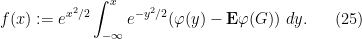
(One could dub

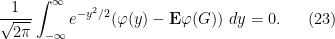
By completing the square, we see that 


which when inserted back into (24) gives the boundedness of
we see on differentiation under the integral sign (and using the Lipschitz nature of 


Applying (24) with 

By the hypothesis (i), the right-hand side goes to zero, hence the left-hand side does also, and the claim follows.
The above theorem gave only a qualitative result (convergence in distribution), but the proof is quite quantitative, and can be used to in particular to give Berry-Esséen type results. To illustrate this, we begin with a strengthening of Theorem 28 that reduces the number of derivatives of
Theorem 31 (Berry-Esséen theorem, less weak form) Let
where

Proof: Set 
Let

We expand 


where ![{[0,1]}](https://s0.wp.com/latex.php?latex=%7B%5B0%2C1%5D%7D&bg=ffffff&fg=000000&s=0&c=20201002)


Another application of independendence gives
so we may rewrite (28) as

Recall from the proof of Theorem 30 that 


and the claim follows from Hölder’s inequality.
This improvement already reduces the 
Theorem 32 (Berry-Esséen theorem, bounded case) Let
whenever
, where

Proof: Write ![{\phi := 1_{(-\infty,a]}}](https://s0.wp.com/latex.php?latex=%7B%5Cphi+%3A%3D+1_%7B%28-%5Cinfty%2Ca%5D%7D%7D&bg=ffffff&fg=000000&s=0&c=20201002)

Let 


and by arguing as in the proof of Theorem 31, we can write the right-hand side as
From (24),

The 
and so we conclude that
Since

applying the second inequality and using independence to once again eliminate the 
which implies (by another appeal to the non-increasing nature of

or in other words that

Similarly, using the lower bound inequalities, one has

Moving 
Actually, one can use Stein’s method to obtain the full Berry-Esséen theorem, but the computations get somewhat technical, requiring an induction on
— 7. Predecessor comparison —
Suppose one had never heard of the normal distribution, but one still suspected the existence of the central limit theorem – thus, one thought that the sequence
Certainly in the case of Bernoulli distributions, one could work explicitly using Stirling’s formula (see Exercise 3), and the Fourier-analytic method would also eventually work. Let us now give a third way to (heuristically) derive the normal distribution as the limit of the central limit theorem. The idea is to compare 

(normalising 


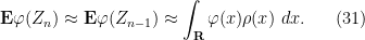
Now let us try to combine this with (30). We assume


Taking expectations, and using the independence of

Up to errors of 


Changing variables for the first term on the right hand side, and integrating by parts for the second term, we have
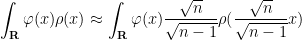
Since

Taylor expansion gives

which leads us to the heuristic ODE

where 

Observe that 

which is (21), and can be solved by standard ODE methods as 

The above argument was not rigorous, but one can make it so with a significant amount of PDE machinery. If we view 

which is a linear parabolic equation that is fortunate enough that it can be solved exactly (indeed, it is not difficult to transform this equation to the linear heat equation by some straightforward changes of variable). Using the spectral theory of the Ornstein-Uhlenbeck operator
This argument does, though highlight two ideas which we will see again in later notes when studying random matrices. Firstly, that it is profitable to study the distribution of some random object

87 comments
Comments feed for this article
6 January, 2010 at 2:02 am
Jean
Very nice notes! Thank you!
Just a remark: in http://arxiv.org/abs/0705.1224 and http://arxiv.org/abs/0908.0391, one can find some applications of Stein’s method in random matrix theory.
6 January, 2010 at 7:27 am
Mark Meckes
More applications of Stein’s method in random matrix theory appear here, here, and here.
6 January, 2010 at 2:53 am
karabasov
A couple of very minor typos:
1) in the second-last paragraph of section 3, it should be “to those terms in (17)”
2) Beginning of section 4: “Lindeberg observed that” – the comma between observed and that is not correct.
6 January, 2010 at 3:25 am
karabasov
I think there might be a parsing error around “where L is the rhox” in the last section… or maybe I just don’t get it.
6 January, 2010 at 9:12 am
Giovanni Peccati
Hi Terry,
thank you for these inspiring lecture notes !
Small typo, in the brackets starting 5 lines after formula (30) (If we secretely…) there is a square root missing in the normalizing factor of the Gaussian density.
Best, G
6 January, 2010 at 12:04 pm
Terence Tao
Thanks for the corrections!
Somewhat embarrassingly, I was only dimly aware of the work on applying Stein’s method to random matrices; it seems that the fraction of literature on the subject that I am familiar with is still not fully representative. Thanks for the references!
7 January, 2010 at 5:45 am
Tim vB
Dear Terry,
thanks for this marvelous lecture notes!
I hope the following two remarks are not too pedantic, but both points made me stop for a short while:
1. The part “now we get the Fokker-Planck-Equation and that can be solved exactly” confused me a bit, because the Fokker-Planck-Equation can “usually” not be solved excatly – the one for the Ornstein-Uhlenbeck process can. It’s of course clear from the context that you mean exactly this, but I think it would help me if you redundantly write ” the above computations heuristically lead us eventually to the Fokker-Planck equation of the Ornstein-Uhlenbeck process”.
2. Wouldn’t most people say the Ornstein-Uhlenbeck process is the solution of a stochastic ordinary differential equation (stochastic ODE) rather than a stochastic partial differential equation?
[Fair enough; I’ve adjusted the notes accordingly.]
15 January, 2010 at 12:31 pm
Steven Heilman
More tedious [potential] corrections:
1. Two Eqs. after Eq. (14): P(…)\leq E(…)
2. Eq (16): square in denominator correct?
3. Theorem 4,5: F should be phi (or vice versa)
4(a). Proof of Theorem 5: several missing parentheses? (or E symbols), e.g.
\displaystyle {\bf E} (\varphi(Z_n) – \varphi(W_n)) = o(1).
This is done quite a lot, so I will assume it was done on purpose.
4(b). telescoping sum, multiply by -1
5. After Eq. (26): tex error for bound on f. I assume you want
{f(x) = O_\varphi( 1/|x|)}
[Corrected, thanks – T.]
17 January, 2010 at 7:28 pm
salazar
Second 1 and 3. For 4, since W_n is a RV, there should be no ambiguity. For 2, I haven’t been able to see how to replace \hat{eta}.
17 January, 2010 at 8:55 pm
Terence Tao
18 January, 2010 at 6:29 pm
254A, Notes 3b: Brownian motion and Dyson Brownian motion « What’s new
[…] the central limit theorem from the fundamental solution of the heat equation (cf. Section 7 of Notes 2), although the derivation is only heuristic because one first needs to know that some limiting […]
29 January, 2010 at 7:16 am
Andreas Naive
Excellent notes!
Just a small fix:
In (30), should be
  , which slightly simplify the following argument.
[Corrected, thanks – T.]
2 February, 2010 at 1:34 pm
254A, Notes 4: The semi-circular law « What’s new
[…] vein, we may apply the truncation argument (much as was done for the central limit theorem in Notes 2) to reduce the semi-circular law to the bounded case: Exercise 5 Show that in order to prove the […]
10 February, 2010 at 10:56 pm
245A, Notes 5: Free probability « What’s new
[…] an interesting analogue in the freely independent setting. For instance, the central limit theorem (Notes 2) for averages of classically independent random variables, which roughly speaking asserts that such […]
25 February, 2010 at 10:19 am
PDEbeginner
Dear Prof. Tao,
I have some problems on Ex 12 (Esseen concentration inequaity) and Thm 3:
Ex 12. Let , the value on LHS of (9) should be 1, while that on RHS should be 0. Then the inequality breaks down.
Thm 3. In the paragraph immediately below (14), I do not understand how to apply an integration by parts argument, since one does not know the exact distribution of .
.
Thanks in advance!
25 February, 2010 at 11:09 am
Terence Tao
Ah, there was a factor of r^d missing in the concentration inequality; it is fixed now.
As for Theorem 3, the point is that the distribution of X is the Stieltjes derivative of the cumulative distribution function of X;
of X;  . If we integrate the latter integral by parts, we see that small perturbations of F in the uniform norm lead to small perturbations of
  when f has bounded total variation.
25 February, 2010 at 10:20 am
PDEbeginner
Sorry, it is Ex 11.
26 February, 2010 at 2:41 pm
YP
The derivation of Gaussian in Section 7 is amazing! (To me it seems very much in the spirit of physics). Isn’t it strange that to our brain it seems very natural to make this argument as it is, whereas for scientific community you actually need to add days of hard work (in Sobolev spaces etc)?
27 February, 2010 at 6:44 pm
vedadi
Dear Prof. Tao,
We know that for i.i.d mean zero, variance one random variables,
  converges in distribution to the point mass at zero,
  and standard normal r.v.
  for
for  respectively. Do we have convergence in distribution for other values
Thanks
6 March, 2010 at 7:14 pm
254A, Notes 7: The least singular value « What’s new
[…] understand this walk, we apply (a slight variant) of the Berry-Esséen theorem from Notes 2: Exercise 1 Show […]
10 March, 2010 at 10:35 am
PDEbeginner
Dear Prof. Tao,
I finished reading this note. As usual, I have some problems :-)
1. For the moment method, we first apply Chernoff bound (3), and then we can assume that are uniformly guassian. But when proving Chernoff bound in Note 1, we have used the identity
  . When we are dealing random matrices, if we also use Chernoff bounds, then it seems we shall have some trouble.
2. I still do not know how to prove the conclusion in Ex 11. Suppose one is trying to bound the easy probability (with and
and  ):
):
By Fourier transform, we obtain
Clearly, to show has the same bound as in exercise, we need to show that
  has that bound. I don’t know to show this.
3. A small typo: the in Theorem 5 seems to be
  .
.
10 March, 2010 at 6:38 pm
Terence Tao
1. For random matrices, one does not apply the Chernoff bound to the matrix directly, but to other scalar expressions related to that matrix, e.g. linear combinations of the matrix entries.
2. One first needs to replace the sharp cutoff to the ball of radius r by a smoother cutoff. This is the method of smoothing sums:
http://www.tricki.org/article/Smoothing_sums
3. Thanks for the correction!
5 May, 2010 at 8:48 pm
Anonymous
These notes are very helpful, thank you very much!
I do not have a strong background in the Fourier analysis, could you point me to a refernce to the solutions to Exercise 11 and Exercise 15?
A few comments I have:
In Exercise 13, the characteristic function should be $e^{i\mu}t…$ instead of $e^{-i\mu}t$?
In Part 1 of this note, the “N” in the last two singled-out equations should be replaced with “N_n”?
6 May, 2010 at 9:06 am
Terence Tao
Thanks for the corrections,’
For Ex11, see Lemma 7.17 of my book “Additive combinatorics” with Van Vu. Ex15 can be found in most graduate texts in probability, including those listed at the link given.
27 July, 2010 at 3:50 pm
Ahmet Arivan
Great notes. I have probably a very stupid question. But in the Stein method section, it is claimed that if f(t) =O(1/1+|t|) and f'(t)=O(1) then tf(t) is Lipschitz with constant of O(1). Is it possible to give a hint on why this is true?
Thanks,
31 July, 2010 at 8:35 am
Terence Tao
Ah yes, that requires an additional argument (which needs the Lipschitz hypothesis on phi). I’ve modified the text accordingly (and in particular weakened the Berry-Esseen type claim, since the Lipschitz property is not present in that case.)
29 October, 2012 at 3:53 pm
Nick Cook
Small thing: I think the last part of the proof of Theorem 6, showing that , with implicit constant linear in the bounded Lipschitz norm of
  , belongs just after this proof since we aren’t assuming
  is Lipschitz here. – or leave it in with modification of the phrase “using the Lipschitz nature of
  ” :)
” :)
[Corrected by assuming $\phi$ to be Lipschitz. -T.]
4 November, 2010 at 8:33 am
Qiaochu Yuan
Regarding Section 7: I had always vaguely figured that if were going to converge to a particular distribution, it would have to converge to an eigenfunction of the Fourier transform. Do you know of any heuristic (or rigorous!) derivations of the CLT using this idea?
4 November, 2010 at 9:02 am
Terence Tao
I think the more accurate statement would be that a stable law should have a Fourier transform whose logarithm is an eigenfunction of the scaling operation, since the convolution
  of
of  with itself needs to be a rescaling of
  .
.
16 November, 2010 at 1:04 pm
karabasov
At the beginning of the proof of theorem 1, it seems that the first “for sufficiently small t” is not needed. Only the second is needed.
15 March, 2011 at 6:57 pm
Sujit
Hi Terry,
I am a bit puzzled about Exercise 1. I am thinking of $Z_n$ as a map from $n$ copies of $\Omega$ to $R$. If this is the case, what does it mean to say $Z_n$ converges almost surely? Isn’t the underlying sample space varying as $n$ varies?
The CLT says something about the push forward of the measures from $\Omega^n$ to $R$ and I can understand it. So even if the sample space changes, it doesn’t matter as we are comparing the push forward measures. In the strong LLN case, it still sounds fine to me if I interpret the almost sure convergence as almost sure convergence to the constant map on $\Omega^n$ given by the expectation. But I am having trouble trying to understand what Exercise 1 means.
Thanks
15 March, 2011 at 7:08 pm
Terence Tao
The intent here is to work in a common extension of all these probability spaces, where we have an infinite sequence of iid random variables (and this is also the correct way to interpret the strong law of large numbers).
16 March, 2011 at 1:03 pm
Anonymous
Dear Prof. Tao,
Let be the moment generating function of a non degenerate r.v
  . Then is
  always strictly increasing and strictly convex on
  ?
?
Thanks
28 August, 2011 at 6:12 am
The law of large numbers and the central limit theorem | Controlled Complexity
[…] theorem (CLT). There are excellent resources on the net for LLN and CLT. For example, this and this are highly recommended readings. This blog will play a complementary with figures and animations to […]
1 October, 2011 at 10:32 am
Anonymous
Can anyone help me to compute the expected waiting time of the first occurrence of the patten, say, TTHT. here
is there a general approach to solve this sort of problems?
Thanks
18 November, 2011 at 2:38 am
Diffusion in Ehrenfest wind-tree model « Disquisitiones Mathematicae
[…] of the word “abnormal” comes by comparison with Brownian motion and/or central limit theorem: once we know that the diffusion is “sublinear” (maybe after removing the […]
17 March, 2012 at 5:48 am
Anonymous
Dear Prof. Tao,
Let be the simple symmetric random walk in one dimension.
 I need a lower bound for the following probability which does not depend on
Assume that K is a large constant and
What is the idea behind finding a lower bound for this type of quantities?
Thank you
10 October, 2012 at 3:33 pm
Robert Kohn
Hi, thanks for insightful presentation. My question is, suppose that the are independent with finite third moments, zero mean and unit variance. What can we say about the convergence of the third moment of the normalized sum ?
 are correlated?
In addition, what results of the same kind can we get if the
Thanks,
Robert Kohn
20 November, 2012 at 8:14 am
Jack
Regarding Exercise 1: I don’t see how the intuition help. What I thought is to give a lower bound of for some
  , which is from the definition of convergence in probability. Could you elaborate the intuition? Why would independence help here?
20 November, 2012 at 8:41 am
Terence Tao
Actually, one needs a lower bound on to contradict convergence in probability to an unspecified limit (lower bounding
  merely prevents convergence in probability to zero, or to a non-positive random variable). But if one can quantify some approximate independence between
  and
and  for n,m widely separated, then this, together with the central limit theorem, can supply the desired lower bound.
20 November, 2012 at 2:07 pm
Jack
An attempt is that both and $Z_{2n}$ converge to
  in distribution by CLT. Thus one has
  . I still don’t see how one can bound
  .
.
20 November, 2012 at 2:14 pm
Terence Tao
20 November, 2012 at 2:46 pm
Jack
What puzzles me is the use of “independence” here. As a beginner, I only think that and
and  are independent if and only if
  where
where  and
and  are Borel sets in the corresponding Borel sigma algebra. Why does this concept have anything to do with the “distance” between these random variables? It’s quite intuitive though: two things are “independent”, then they should not be too “close” to each other. But I don’t see the connection. (Eventually I come up with something like
  . Is this the point? )
20 November, 2012 at 6:24 pm
Terence Tao
If X and Y are independent, then (for instance) will be large if
  and
and  are large, thus giving some separation between X and Y. (One can also in principle work with expectations, but this requires some hypotheses on absolute integrability that one then has to justify separately.)
26 November, 2012 at 3:13 pm
Jack
Finding a lower bound for is still not “obvious” to me. I tried
  . And the independence between
  and
and  gives
gives  . Since
  is chosen such that
  ,
,  implies that this is very close to the desired estimate. But I don’t see the way to bound
  and
and  . Since I haven’t use CLT so far, I am wondering there must be lack of something here.
26 November, 2012 at 3:42 pm
Terence Tao
The CLT describes the limiting value of in the limit as
  with
with  fixed, and similarly for
  (which is basically a rescaled variant of
  ).
).
26 November, 2012 at 4:14 pm
Jack
I found in some book that random variables converging in distribution to $X$ is defined as (and the author also calls it “weak convergence”)
 for all bounded, continuous function
  . Is it “equivalent” to the definition in [254A Note4 Exercise 18](https://terrytao.wordpress.com/2010/10/02/245a-notes-4-modes-of-convergence/)? But in [245B Note 11](https://terrytao.wordpress.com/2009/02/21/245b-notes-11-the-strong-and-weak-topologies/), weak convergence is convergence in weak topology. I am totally confused with the terminologies.
[I don’t know how to give links like people do in MathOverflow.]
26 November, 2012 at 4:39 pm
Terence Tao
Yes, these notions are all connected to each other; see Exercise 23 of https://terrytao.wordpress.com/2010/01/01/254a-notes-0-a-review-of-probability-theory/ . (Though, strictly speaking, vague convergence of measures – which is equivalent to convergence in distribution – is an example of weak* convergence rather than weak convergence.)
22 March, 2013 at 12:34 am
Anonymous
Hi professor Tao,
does the CLT hold if we substitute the hypothesis of finite mean and variance with the hypothesis of finite second order moment, ?
?
22 March, 2013 at 9:10 am
Terence Tao
By Holder’s inequality (or the Cauchy-Schwarz inequality), finite second order moment is equivalent to finite mean and variance.
3 April, 2013 at 3:13 am
Anonymous
Thanks a lot for the answer! By the way, does { \Z_n := \frac{S_n – n \mu}{\sqrt{n} \sigma} to N(0,1)} implies that {\frac{S_n}{n} to N(\mu,\frac{\sigma^2}{n}) }? This implication seems quite weird to me, since {n to \infty}, but on a book about generalized polynomial chaos I fount the following sentence: “the numerical average of a sequence of i.i.d. random variables will converge, as n is increased, to a Gaussian distribution { N(\mu,\frac{\sigma^2}{n}) } […]”.
3 April, 2013 at 10:30 am
Terence Tao
If one uses a rescaled notion of convergence, then this statement is true, although if one uses unrescaled versions of convergence (e.g. convergence in distribution, vague convergence, total variation convergence, etc.) then the statement is either false or trivially true, depending on exactly which mode of convergence is specified. It is somewhat of an abuse of notation to refer to convergence of random variables without specifying the exact nature of the convergence, although for informal mathematical discussion it is generally permissible to be a bit loose in this regard.
7 May, 2013 at 3:44 am
Anonymous
(i) In Remark 1 the word theorem is missing from “central limit theorem.”
(ii) The equation following the sentence “From the bounded density of $G$ and the rapid decrease of $\eta$ we have…” I think the first term should be an expectation and not probability.
(iii) Do you use any convention for capitalizing theorems? For example, you write “central limit theorem” in lower case but “Taylor” expansion in upper case.
(iv) What is the diagonalisation argument in “By a diagonalisation argument, we conclude that there exists a sequence…”? Is there a Wikipedia page? Thanks.
[Corrected, thanks. Taylor is a proper noun and is therefore capitalised in English. The diagonalisation argument, originally due to Cantor, refers to any procedure in which one repeatedly extracts sequences with various properties and then passes to a diagonal subsequence with an even better property. Actually, the Arzela-Ascoli diagonalisation argument is closer in spirit to the one used here than the Cantor diagonalisation argument.]
13 May, 2013 at 12:00 pm
חסם צ'רנוף, חסם אנטרופיה ומה שביניהם | One and One
[…] נדבר עליו כאן, אתם מוזמנים לקרוא עליו בבלוג של טרי טאו. אבל גם אם פשוט נאמין שהאינטגרל הזה קרוב מספיק […]
2 November, 2015 at 7:06 pm
275A, Notes 4: The central limit theorem | What's new
[…] theorem (including some further proofs, such as one based on Stein’s method) can be found in this blog post. Some further variants of the central limit theorem, such as local limit theorems, stable laws, and […]
28 December, 2015 at 5:32 am
Vladimir
Dear Tao, I do not get it why in the proof of theorem 7 the t is uniformly distributed even if independence of Z_n:i is clear to me? Could you help please?
28 December, 2015 at 8:14 am
Terence Tao
which is of course a special case of the fundamental theorem of calculus.
29 December, 2015 at 2:49 am
Vladimir
Many thanks, now I get it.
27 January, 2016 at 8:50 am
Anonymous
Dear Prof. Tao, in exercise 8, shouldn’t the derivative be evaluated at 0?
[Exercise reworded – T.]
3 May, 2016 at 2:41 pm
Vivek Kumar Bagaria
Great notes! How does the ‘Vector-valued central limit’ behave if the dimension of the vector scales with the number of samples $n$ ?
4 May, 2016 at 8:30 am
Terence Tao
This basically comes down to the dependence of constants of the Berry-Esseen theorem on dimension. The best bound I know of in this direction comes from this 2003 paper of Bentkus, but there may be further improvements since then.
5 May, 2016 at 4:11 am
easy
why is the third moment important in that paper? CLT is about second moments right?
5 May, 2016 at 8:12 am
Terence Tao
If one just wants qualitative convergence (with no rate), then second moment conditions suffice, but in order to obtain quantitative bounds one needs some higher moment assumption (to deal with the errors caused by truncation arguments). Also one can get faster rates of convergence than Berry-Esseen if the original distribution matches third or higher moments with the gaussian, as can be seen from the Lindeberg argument (or from the Fourier argument).
7 November, 2016 at 10:26 pm
Sahiba
Hey, can you help me in Exercise 1? I’m not able to solve it.
8 February, 2017 at 10:10 pm
John Rawls
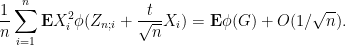
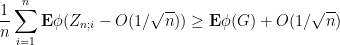
These notes are immensely useful as always, but I have a small question: how exactly does the diagonalization argument in Section 1 work? We know that![\lim_{n\to\infty}\mathbb{E}[f(Z_{n,\leq N})]=\mathbb{E}[f(G)]](https://s0.wp.com/latex.php?latex=%5Clim_%7Bn%5Cto%5Cinfty%7D%5Cmathbb%7BE%7D%5Bf%28Z_%7Bn%2C%5Cleq+N%7D%29%5D%3D%5Cmathbb%7BE%7D%5Bf%28G%29%5D&bg=ffffff&fg=545454&s=0&c=20201002) for each fixed
for each fixed  and all bounded continuous
  , but it seems that the rate of convergence depends not only on
  but also on
  . How then can we choose
  so that we get
 ![\lim_{n\to\infty}\mathbb{E}[f(Z_{n,\leq N_n})]=\mathbb{E}[f(G)]](https://s0.wp.com/latex.php?latex=%5Clim_%7Bn%5Cto%5Cinfty%7D%5Cmathbb%7BE%7D%5Bf%28Z_%7Bn%2C%5Cleq+N_n%7D%29%5D%3D%5Cmathbb%7BE%7D%5Bf%28G%29%5D&bg=ffffff&fg=545454&s=0&c=20201002) for all
for all  , or at least for all
  in some nice subclass? Thanks!
9 February, 2017 at 10:27 pm
Terence Tao
One can work with some countable dense sequence of functions (e.g. indicator functions of
  with
with  an enumeration of the rationals will work). For each
  , we then can find
  such that
  lies within
  of
of  for all
  and
and  ; we can also ensure that the
  are increasing in
  . Letting
  be the inverse of
  (or more precisely,
  is the first
  for which
  ) we see that
  for all
  , and by approximating a general
  using the
  we obtain convergence in distribution.
14 February, 2017 at 8:32 pm
John Rawls
Very clever, thank you!
16 February, 2017 at 10:07 am
tpfly
Hi professor Tao,
I’m reading this series of notes and I have a question about the proof of Berry Esseen Theorem. You said that in order to establish (13) it suffices to establish (15) because of (8). But (8) requires that $\varphi$ is Schwartz, or at least L1 and the fourier transform should be also L1, because the Fourier inverse is used. However the function in the proof of berry esseen is decreasing from $1$ to $0$, is (8) still available with this kind of functions?
Thanks!
17 February, 2017 at 5:34 am
tpfly
I found the answer of my question by taking a limit, that is,![\mathbb{E}\varphi(X-a)=\lim_{T\to +\infty}\mathbb{E}[\varphi(X-a)-\varphi(X+T)]](https://s0.wp.com/latex.php?latex=%5Cmathbb%7BE%7D%5Cvarphi%28X-a%29%3D%5Clim_%7BT%5Cto+%2B%5Cinfty%7D%5Cmathbb%7BE%7D%5B%5Cvarphi%28X-a%29-%5Cvarphi%28X%2BT%29%5D&bg=ffffff&fg=545454&s=0&c=20201002) and now the expectation is taken on a Schwartz function.
and now the expectation is taken on a Schwartz function.
By the way I think there are some mistakes in this proof, the Fourier transform
![\displaystyle \hat 1_{-\infty,a]}=O(\frac{1}{1+|t|})](https://s0.wp.com/latex.php?latex=%5Cdisplaystyle+%5Chat+1_%7B-%5Cinfty%2Ca%5D%7D%3DO%28%5Cfrac%7B1%7D%7B1%2B%7Ct%7C%7D%29&bg=ffffff&fg=545454&s=0&c=20201002)
![\displaystyle \hat 1_{-\infty,a]}=O(\frac{1}{|t|})](https://s0.wp.com/latex.php?latex=%5Cdisplaystyle+%5Chat+1_%7B-%5Cinfty%2Ca%5D%7D%3DO%28%5Cfrac%7B1%7D%7B%7Ct%7C%7D%29&bg=ffffff&fg=545454&s=0&c=20201002)
![\int1_{-\infty,a]}](https://s0.wp.com/latex.php?latex=%5Cint1_%7B-%5Cinfty%2Ca%5D%7D&bg=ffffff&fg=545454&s=0&c=20201002) would be finite. And
would be finite. And
![\displaystyle \hat \varphi(t) = \hat 1_{(-\infty,a]}(t) \hat \eta(t/\epsilon)](https://s0.wp.com/latex.php?latex=%5Cdisplaystyle+%5Chat+%5Cvarphi%28t%29+%3D+%5Chat+1_%7B%28-%5Cinfty%2Ca%5D%7D%28t%29+%5Chat+%5Ceta%28t%2F%5Cepsilon%29&bg=ffffff&fg=545454&s=0&c=20201002)
![\displaystyle \hat \varphi(t) = \hat 1_{(-\infty,a]}(t) \hat \eta(t\epsilon)](https://s0.wp.com/latex.php?latex=%5Cdisplaystyle+%5Chat+%5Cvarphi%28t%29+%3D+%5Chat+1_%7B%28-%5Cinfty%2Ca%5D%7D%28t%29+%5Chat+%5Ceta%28t%5Cepsilon%29&bg=ffffff&fg=545454&s=0&c=20201002) .
.
should be
as there must be a singular point at 0, otherwise
should be
[New version of proof given – T.]
6 July, 2017 at 2:45 pm
Syntactic Translations of Berry-Esséen and the CLT | Polynomially Bounded
[…] noted in Remark 29 here, one can improve the constant term by changing the replacement variables. In particular, it […]
21 December, 2017 at 2:13 am
Nick Cook
A couple of typos in the proof of Theorem 23: In the first display after (15) it should say (with no change to (16)), and above the last display it should say “if
  “.
“.
[Corrected, thanks – T.]
15 April, 2018 at 12:36 am
Ankit
Hi Prof. Tao,
Thanks for the wonderful notes. These are great for self-studying.
In Eq. (17), shouldn’t there be a summation over different choices of {a_1,\ldots,a_m} as well? cf. with the case of k = 4 where terms are explicitly written.
It doesn’t affect the result in the end though because all of them have to be 2 for the non-vanishing term.
15 April, 2018 at 9:14 am
Terence Tao
One is summing over all choices of and of
  , yes (see the text immediately before and after (17)).
15 April, 2018 at 11:03 am
Ankit
I see. Thank you for replying.
20 April, 2018 at 8:49 pm
Damodar
Prof. Tao, I would be very glad if you could look at my blog post on ” A full proof of Berry-Esseen inequality in the Central Limit Theorem”.
Description: This theorem gives us the maximum convergence limit of the basin of attraction in the Central limit theorem.
Link: http://www.physicslog.com/proof-berry-essen-theorem/
Thanks,
Damodar
3 June, 2018 at 11:51 am
Anonymous
Dear Prof Tao, I have a question about the proof using the Fourier method. The proof (around equation (11)) only uses $t$ in a neighborhood of the origin. My question is if this is equivalent to independence (i.e., does $F_{X,Y}(t,s)=F_X(t)F_Y(t)$ for $t$ in a neighborhood of the origin imply $F_{X,Y}(t,s)=F_X(t)F_Y(t)$ for all $t \in V$)? Thanks.
4 June, 2018 at 10:14 pm
Terence Tao
If are bounded (or subgaussian) random variables, then
  are analytic functions of
  , and so by analytic continuation any identity that holds for small
  automatically holds for large
  . I don’t know what happens though if
  are more heavy-tailed, there may well be (somewhat artificial) counterexamples in this setting.
15 February, 2020 at 1:47 pm
Anonymous
Dear Prof. Tao, Do you know if there are quantitative versions of local central limit theorems, akin to the Berry-Esseen inequality? I am in particular interested in bounded integer i.i.d. random variables, assuming the number-theoretic issues are not a problem, i.e. the gcd is 1. E.g. think uniform distribution on the set of squares of integers in an interval.
9 March, 2022 at 9:49 am
Aditya Guha Roy
Prof. Tao in Exercise 2 is Kolmogorov’s zero-one law the main thing that works behind the scenes: passing on to a subsequence it suffices to consider only almost sure convergence of a subsequence, but then we see that the normalized sums have mean zero and variance one so the limiting random variable would also have variance one, however since these is a sequence of tail random variables so if it converges in the almost sure sense then the limit must be a constant with probability one and will hence have zero variance, a contradiction which refutes our assumption and hence proves the claim.
Is this correct in your opinion?
[This is indeed one way to solve the exercise – T.]
16 May, 2022 at 2:23 pm
Michael Neely
In the “Random Matrix” book Exercise 1.1.10, what answer did you have in mind? The question may need some fixes, a counter-example seems to be when is uniformly distributed over
 ![[0,1]](https://s0.wp.com/latex.php?latex=%5B0%2C1%5D&bg=ffffff&fg=545454&s=0&c=20201002) ,
, ![X(Omega) = [0,1]](https://s0.wp.com/latex.php?latex=X%28Omega%29+%3D+%5B0%2C1%5D&bg=ffffff&fg=545454&s=0&c=20201002) , and
, and  , so
, so  and
and  have the same distribution but
  cannot be 1/2 so we cannot have
  .
.
16 May, 2022 at 5:29 pm
Michael Neely
By the way this is a stackexchange question here (I gave some preliminary comments on thoughts on the posting of HangY) https://math.stackexchange.com/questions/4450636/distribution-of-a-random-variable-exercise/4450746#4450746
17 May, 2022 at 9:27 am
Terence Tao
Oops, you are right, the exercise is not correct as stated. (On standard probability spaces one can salvage it up to almost sure agreement by using a relative product construction, but this is not the point I wanted to make in this exercise.) I have added an erratum replacing the exercise by one which makes the desired point.
17 May, 2022 at 3:28 pm
Michael Neely
Thanks for the quick reply! However, I don’t think this works. I believe I can construct two independent random variables![X_i:Omega\rightarrow\mathbb[0,1]](https://s0.wp.com/latex.php?latex=X_i%3AOmega%5Crightarrow%5Cmathbb%5B0%2C1%5D&bg=ffffff&fg=545454&s=0&c=20201002) for
for  , both uniformly distributed over
 ![[0,1]](https://s0.wp.com/latex.php?latex=%5B0%2C1%5D&bg=ffffff&fg=545454&s=0&c=20201002) , such that the intersection of their images
, such that the intersection of their images  is the empty set. If I understand your updated question properly, this is a (counterintuitive) counter example to your claim.
17 May, 2022 at 5:15 pm
Michael Neely
Nevermind, I think my counterexample might be circumvented by your “almost surely” insertion (taken on the probability spaces, rather than on the R space) if we give different parts of the two different spaces measure 0 with respect to the different measures.