Let us call an arithmetic function 
 -bounded if we have
  for all
  . In this section we focus on the asymptotic behaviour of -bounded multiplicative functions. Some key examples of such functions include:
- The Möbius function
 ;
;
- The Liouville function
 ;
;
- “Archimedean” characters
 (which I call Archimedean because they are pullbacks of a Fourier character
  on the multiplicative group
  , which has the Archimedean property);
- Dirichlet characters (or “non-Archimedean” characters)
 (which are essentially pullbacks of Fourier characters on a multiplicative cyclic group
  with the discrete (non-Archimedean) metric);
- Hybrid characters
 .
.
The space of -bounded multiplicative functions is also closed under multiplication and complex conjugation.
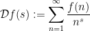
Given a multiplicative function  , we are often interested in the asymptotics of long averages such as

for large values of  , as well as short sums
where  and
and  are both large, but is significantly smaller than . (Throughout these notes we will try to normalise most of the sums and integrals appearing here as averages that are trivially bounded by
  ; note that other normalisations are preferred in some of the literature cited here.) For instance, as we established in Theorem 58 of Notes 1, the prime number theorem is equivalent to the assertion that

as  . The Liouville function behaves almost identically to the Möbius function, in that estimates for one function almost always imply analogous estimates for the other:
Exercise 1 Without using the prime number theorem, show that (1) is also equivalent to
as . (Hint: use the identities  and
and  .)
.)
Henceforth we shall focus our discussion more on the Liouville function, and turn our attention to averages on shorter intervals. From (2) one has

as  if
if  is such that
  for some fixed
  . However it is significantly more difficult to understand what happens when grows much slower than this. By using the techniques based on zero density estimates discussed in Notes 6, it was shown by Motohashi and that one can also establish \eqref. On the Riemann Hypothesis Maier and Montgomery lowered the threshold to
  for an absolute constant
  (the bound
  is more classical, following from Exercise 33 of Notes 2). On the other hand, the randomness heuristics from Supplement 4 suggest that should be able to be taken as small as
  , and perhaps even
  if one is particularly optimistic about the accuracy of these probabilistic models. On the other hand, the Chowla conjecture (mentioned for instance in Supplement 4) predicts that cannot be taken arbitrarily slowly growing in , due to the conjectured existence of arbitrarily long strings of consecutive numbers where the Liouville function does not change sign (and in fact one can already show from the known partial results towards the Chowla conjecture that (3) fails for some sequence and some sufficiently slowly growing , by modifying the arguments in these papers of mine).
The situation is better when one asks to understand the mean value on almost all short intervals, rather than all intervals. There are several equivalent ways to formulate this question:
Exercise 2 Let  be a function of such that
  and
and  as . Let be a -bounded function. Show that the following assertions are equivalent:
As it turns out the second moment formulation in (iii) will be the most convenient for us to work with in this set of notes, as it is well suited to Fourier-analytic techniques (and in particular the Plancherel theorem).
Using zero density methods, for instance, it was shown by Ramachandra that

whenever  and . With this quality of bound (saving arbitrary powers of
  over the trivial bound of ), this is still the lowest value of one can reach unconditionally. However, in a striking recent breakthrough, it was shown by Matomaki and Radziwill that as long as one is willing to settle for weaker bounds (saving a small power of or
  , or just a qualitative decay of
  ), one can obtain non-trivial estimates on far shorter intervals. For instance, they show
Theorem 3 (Matomaki-Radziwill theorem for Liouville) For any  , one has
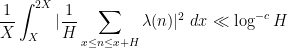
for some absolute constant  .
.
In fact they prove a slightly more precise result: see Theorem 1 of that paper. In particular, they obtain the asymptotic (4) for any function that goes to infinity as , no matter how slowly! This ability to let grow slowly with is important for several applications; for instance, in order to combine this type of result with the entropy decrement methods from Notes 9, it is essential that be allowed to grow more slowly than . See also this survey of Soundararajan for further discussion.
Exercise 4 In this exercise you may use Theorem 3 freely.
(There is a curious asymmetry to the difficulty level of these bounds; the upper bound in (ii) was established much earlier by Harman, Pintz, and Wolke, but the lower bound in (i) was only established in the Matomaki-Radziwill paper.)
The techniques discussed previously were highly complex-analytic in nature, relying in particular on the fact that functions such as or have Dirichlet series  ,
,  that extend meromorphically into the critical strip. In contrast, the Matomaki-Radziwill theorem does not rely on such meromorphic continuations, and in fact holds for more general classes of -bounded multiplicative functions , for which one typically does not expect any meromorphic continuation into the strip. Instead, one can view the Matomaki-Radziwill theory as following the philosophy of a slightly different approach to multiplicative number theory, namely the pretentious multiplicative number theory of Granville and Soundarajan (as presented for instance in their draft monograph). A basic notion here is the pretentious distance between two -bounded multiplicative functions
  (at a given scale ), which informally measures the extent to which “pretends” to be like
  (or vice versa). The precise definition is
Definition 5 (Pretentious distance) Given two -bounded multiplicative functions , and a threshold  , the pretentious distance
  between and up to scale is given by the formula

Note that one can also define an infinite version  of this distance by removing the constraint
  , though in such cases the pretentious distance may then be infinite. The pretentious distance is not quite a metric (because
  can be non-zero, and furthermore can vanish without being equal), but it is still quite close to behaving like a metric, in particular it obeys the triangle inequality; see Exercise 16 below. The philosophy of pretentious multiplicative number theory is that two -bounded multiplicative functions will exhibit similar behaviour at scale if their pretentious distance is bounded, but will become uncorrelated from each other if this distance becomes large. A simple example of this philosophy is given by the following “weak Halasz theorem”, proven in Section 2:
Proposition 6 (Logarithmically averaged version of Halasz) Let be sufficiently large. Then for any -bounded multiplicative functions , one has

for an absolute constant .
In particular, if does not pretend to be , then the logarithmic average  will be small. This condition is basically necessary, since of course
  .
.
If one works with non-logarithmic averages  , then not pretending to be is insufficient to establish decay, as was already observed in Exercise 11 of Notes 1: if is an Archimedean character
  for some non-zero real
  , then goes to zero as (which is consistent with Proposition 6), but does not go to zero. However, this is in some sense the “only” obstruction to these averages decaying to zero, as quantified by the following basic result:
Theorem 7 (Halasz’s theorem) Let be sufficiently large. Then for any -bounded multiplicative function , one has
for an absolute constant and any  .
.
Informally, we refer to a -bounded multiplicative function as “pretentious’; if it pretends to be a character such as  , and “non-pretentious” otherwise. The precise distinction is rather malleable, as the precise class of characters that one views as “obstructions” varies from situation to situation. For instance, in Proposition 6 it is just the trivial character which needs to be considered, but in Theorem 7 it is the characters with
  . In other contexts one may also need to add Dirichlet characters
  or hybrid characters such as
  to the list of characters that one might pretend to be. The division into pretentious and non-pretentious functions in multiplicative number theory is faintly analogous to the division into major and minor arcs in the circle method applied to additive number theory problems; see Notes 8. The Möbius and Liouville functions are model examples of non-pretentious functions; see Exercise 24.
In the contrapositive, Halasz’ theorem can be formulated as the assertion that if one has a large mean
for some  , then one has the pretentious property

for some  . This has the flavour of an “inverse theorem”, of the type often found in arithmetic combinatorics.
Among other things, Halasz’s theorem gives yet another proof of the prime number theorem (1); see Section 2.
We now give a version of the Matomaki-Radziwill theorem for general (non-pretentious) multiplicative functions that is formulated in a similar contrapositive (or “inverse theorem”) fashion, though to simplify the presentation we only state a qualitative version that does not give explicit bounds.
Theorem 8 ((Qualitative) Matomaki-Radziwill theorem) Let  , and let
  , with sufficiently large depending on
  . Suppose that is a -bounded multiplicative function such that

Then one has

for some  .
.
The condition is basically optimal, as the following example shows:
Exercise 9 Let be a sufficiently small constant, and let be such that  . Let be the Archimedean character for some
  . Show that

Combining Theorem 8 with standard non-pretentiousness facts about the Liouville function (see Exercise 24), we recover Theorem 3 (but with a decay rate of only rather than  ). We refer the reader to the original paper of Matomaki-Radziwill (as well as this followup paper with myself) for the quantitative version of Theorem 8 that is strong enough to recover the full version of Theorem 3, and which can also handle real-valued pretentious functions.
With our current state of knowledge, the only arguments that can establish the full strength of Halasz and Matomaki-Radziwill theorems are Fourier analytic in nature, relating sums involving an arithmetic function with its Dirichlet series
which one can view as a discrete Fourier transform of (or more precisely of the measure  , if one evaluates the Dirichlet series on the right edge
  of the critical strip). In this aspect, the techniques resemble the complex-analytic methods from Notes 2, but with the key difference that no analytic or meromorphic continuation into the strip is assumed. The key identity that allows us to pass to Dirichlet series is the following variant of Proposition 7 of Notes 2:
Proposition 10 (Parseval type identity) Let  be finitely supported arithmetic functions, and let
  be a Schwartz function. Then

where  is the Fourier transform of
  . (Note that the finite support of and the Schwartz nature of
  ensure that both sides of the identity are absolutely convergent.)
The restriction that be finitely supported will be slightly annoying in places, since most multiplicative functions will fail to be finitely supported, but this technicality can usually be overcome by suitably truncating the multiplicative function, and taking limits if necessary.
Proof: By expanding out the Dirichlet series, it suffices to show that
for any natural numbers  . But this follows from the Fourier inversion formula
  applied at
  .
. 
For applications to Halasz type theorems, one sets  equal to the Kronecker delta
  , producing weighted integrals of
  of “
of “ ” type. For applications to Matomaki-Radziwill theorems, one instead sets
  , and more precisely uses the following corollary of the above proposition, to obtain weighted integrals of
  of “
of “ ” type:
Exercise 11 (Plancherel type identity) If is finitely supported, and  is a Schwartz function, establish the identity

In contrast, information about the non-pretentious nature of a multiplicative function will give “pointwise” or “ ” type control on the Dirichlet series , as is suggested from the Euler product factorisation of
  .
.
It will be convenient to formalise the notion of , , and control of the Dirichlet series , which as previously mentioned can be viewed as a sort of “Fourier transform” of :
Definition 12 (Fourier norms) Let be finitely supported, and let  be a bounded measurable set. We define the Fourier norm
the Fourier norm

and the Fourier norm
One could more generally define  norms for other exponents
  , but we will only need the exponents
  in this current set of notes. It is clear that all the above norms are in fact (semi-)norms on the space of finitely supported arithmetic functions.
As mentioned above, Halasz’s theorem gives good control on the Fourier norm for restrictions of non-pretentious functions to intervals:
Exercise 13 (Fourier control via Halasz) Let be a -bounded multiplicative function, let  be an interval in
 ![{[C^{-1} X, CX]}](https://s0.wp.com/latex.php?latex=%7B%5BC%5E%7B-1%7D+X%2C+CX%5D%7D&bg=ffffff&fg=000000&s=0&c=20201002) for some
for some  , let
, let  , and let be a bounded measurable set. Show that

(Hint: you will need to use summation by parts (or an equivalent device) to deal with a  weight.)
Meanwhile, the Plancherel identity in Exercise 11 gives good control on the Fourier norm for functions on long intervals (compare with Exercise 2 from Notes 6):
Exercise 14 ( mean value theorem) Let  , and let be finitely supported. Show that
![\displaystyle \| f \|_{FL^2([-T,T])}^2 \ll \sum_n \frac{1}{n} (\frac{T}{n} \sum_{m: |n-m| \leq n/T} |f(m)|)^2.](https://s0.wp.com/latex.php?latex=%5Cdisplaystyle+%5C%7C+f+%5C%7C_%7BFL%5E2%28%5B-T%2CT%5D%29%7D%5E2+%5Cll+%5Csum_n+%5Cfrac%7B1%7D%7Bn%7D+%28%5Cfrac%7BT%7D%7Bn%7D+%5Csum_%7Bm%3A+%7Cn-m%7C+%5Cleq+n%2FT%7D+%7Cf%28m%29%7C%29%5E2.&bg=ffffff&fg=000000&s=0&c=20201002)
Conclude in particular that if is supported in ![{[C^{-1} N, C N]}](https://s0.wp.com/latex.php?latex=%7B%5BC%5E%7B-1%7D+N%2C+C+N%5D%7D&bg=ffffff&fg=000000&s=0&c=20201002) for some
for some  and
and  , then
![\displaystyle \| f \|_{FL^2([-T,T])}^2 \ll C^{O(1)} \frac{1}{N} \sum_n |f(n)|^2.](https://s0.wp.com/latex.php?latex=%5Cdisplaystyle+%5C%7C+f+%5C%7C_%7BFL%5E2%28%5B-T%2CT%5D%29%7D%5E2+%5Cll+C%5E%7BO%281%29%7D+%5Cfrac%7B1%7D%7BN%7D+%5Csum_n+%7Cf%28n%29%7C%5E2.&bg=ffffff&fg=000000&s=0&c=20201002)
In the simplest case of the logarithmically averaged Halasz theorem (Proposition 6), Fourier estimates are already sufficient to obtain decent control on the (weighted) Fourier type expressions that show up. However, these estimates are not enough by themselves to establish the full Halasz theorem or the Matomaki-Radziwill theorem. To get from Fourier control to Fourier or control more efficiently, the key trick is use Hölder’s inequality, which when combined with the basic Dirichlet series identity

gives the inequalities

and

The strategy is then to factor (or approximately factor) the original function as a Dirichlet convolution (or average of convolutions) of various components, each of which enjoys reasonably good Fourier or estimates on various regions  , and then combine them using the Hölder inequalities (5), (6) and the triangle inequality. For instance, to prove Halasz’s theorem, we will split into the Dirichlet convolution of three factors, one of which will be estimated in
  using the non-pretentiousness hypothesis, and the other two being estimated in
  using Exercise 14. For the Matomaki-Radziwill theorem, one uses a significantly more complicated decomposition of into a variety of Dirichlet convolutions of factors, and also splits up the Fourier domain
 ![{[-T,T]}](https://s0.wp.com/latex.php?latex=%7B%5B-T%2CT%5D%7D&bg=ffffff&fg=000000&s=0&c=20201002) into several subregions depending on whether the Dirichlet series associated to some of these components are large or small. In each region and for each component of these decompositions, all but one of the factors will be estimated in , and the other in ; but the precise way in which this is done will vary from component to component. For instance, in some regions a key factor will be small in by construction of the region; in other places, the control will come from Exercise 13. Similarly, in some regions, satisfactory control is provided by Exercise 14, but in other regions one must instead use “large value” theorems (in the spirit of Proposition 9 from Notes 6), or amplify the power of the standard mean value theorems by combining the Dirichlet series with other Dirichlet series that are known to be large in this region.
into several subregions depending on whether the Dirichlet series associated to some of these components are large or small. In each region and for each component of these decompositions, all but one of the factors will be estimated in , and the other in ; but the precise way in which this is done will vary from component to component. For instance, in some regions a key factor will be small in by construction of the region; in other places, the control will come from Exercise 13. Similarly, in some regions, satisfactory control is provided by Exercise 14, but in other regions one must instead use “large value” theorems (in the spirit of Proposition 9 from Notes 6), or amplify the power of the standard mean value theorems by combining the Dirichlet series with other Dirichlet series that are known to be large in this region.
There are several ways to achieve the desired factorisation. In the case of Halasz’s theorem, we can simply work with a crude version of the Euler product factorisation, dividing the primes into three categories (“small”, “medium”, and “large” primes) and expressing as a triple Dirichlet convolution accordingly. For the Matomaki-Radziwill theorem, one instead exploits the Turan-Kubilius phenomenon (Section 5 of Notes 1, or Lemma 2 of Notes 9)) that for various moderately wide ranges ![{[P,Q]}](https://s0.wp.com/latex.php?latex=%7B%5BP%2CQ%5D%7D&bg=ffffff&fg=000000&s=0&c=20201002) of primes, the number of prime divisors of a large number
of primes, the number of prime divisors of a large number  in the range is almost always close to
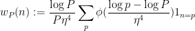
  . Thus, if we introduce the arithmetic functions
![\displaystyle w_{[P,Q]}(n) = \frac{1}{\log\log Q - \log\log P} \sum_{P \leq p \leq Q} 1_{n=p} \ \ \ \ \ (7)](https://s0.wp.com/latex.php?latex=%5Cdisplaystyle+w_%7B%5BP%2CQ%5D%7D%28n%29+%3D+%5Cfrac%7B1%7D%7B%5Clog%5Clog+Q+-+%5Clog%5Clog+P%7D+%5Csum_%7BP+%5Cleq+p+%5Cleq+Q%7D+1_%7Bn%3Dp%7D+%5C+%5C+%5C+%5C+%5C+%287%29&bg=ffffff&fg=000000&s=0&c=20201002)
then we have
![\displaystyle 1 \approx 1 * w_{[P,Q]}](https://s0.wp.com/latex.php?latex=%5Cdisplaystyle+1+%5Capprox+1+%2A+w_%7B%5BP%2CQ%5D%7D&bg=ffffff&fg=000000&s=0&c=20201002)
and more generally we have a twisted approximation
![\displaystyle f \approx f * fw_{[P,Q]}](https://s0.wp.com/latex.php?latex=%5Cdisplaystyle+f+%5Capprox+f+%2A+fw_%7B%5BP%2CQ%5D%7D&bg=ffffff&fg=000000&s=0&c=20201002)
for multiplicative functions . (Actually, for technical reasons it will be convenient to work with a smoothed out version of these functions; see Section 3.) Informally, these formulas suggest that the “ energy” of a multiplicative function is concentrated in those regions where ![{f w_{[P,Q]}}](https://s0.wp.com/latex.php?latex=%7Bf+w_%7B%5BP%2CQ%5D%7D%7D&bg=ffffff&fg=000000&s=0&c=20201002) is extremely large in a sense. Iterations of this formula (or variants of this formula, such as an identity due to Ramaré) will then give the desired (approximate) factorisation of .
is extremely large in a sense. Iterations of this formula (or variants of this formula, such as an identity due to Ramaré) will then give the desired (approximate) factorisation of .
— 1. Pretentious distance —
In this section we explore the notion of pretentious distance. The following Hilbert space lemma will be useful for establishing the triangle inequality for this distance:
Lemma 15 (Triangle inequality) Let  be vectors in a real Hilbert space with
  . Then

Proof: First suppose that are unit vectors:  . Then by the cosine rule
  , and similarly for
  and
and  . The claim now follows from the usual triangle inequality
  .
.
Now suppose we are in the general case when  . In this case we extend to unit vectors by working in the product
  of with the Euclidean space
  and applying the previous inequality to the extended unit vectors


observing that the extensions have the same inner products as the original vectors.
Exercise 16 (Basic properties of pretentious distance) Let  be -bounded multiplicative functions, and let
  .
.
Exercise 17 If  are Dirichlet characters of periods
  respectively induced from the same primitive character, and
  , show that
  for some absolute constant
  (the only purpose of which is to keep the triple logarithm
  positive). (Hint: control the contributions of the primes in each dyadic block
  separately for
  .)
.)
Next, we relate pretentious distance to the value of Dirichlet series just to the right of the critical strip. There is an annoying minor technicality that the prime  has to be treated separately, but this will not cause too much trouble.
Lemma 18 (Dirichlet series and pretentious distance) Let be a -bounded multiplicative function,  , and
, and  . Then


In particular, we always have the upper bound

and if one imposes the technical condition that either  for all
  or
or  for all
  , then

If  for all
  and
and  , then we may delete the
  terms in the above claims.
Proof: By replacing with  we may assume without loss of generality that
  . We begin with the first claim (8). By expanding out the Euler product, the left-hand side of (8) is equal to
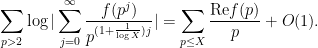
and from Definition 5 and Mertens’ theorem we have

and so it will suffice on canceling the  factor and taking logarithms to show that
For  , the quantity
  differs from by at most
  . Also we have
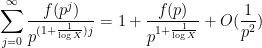
and hence by Taylor expansion
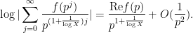
By the triangle inequality, it thus suffices to show that
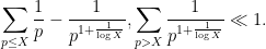
But the first bound follows from the mean value estimate  and Mertens’ theorems, while the second bound follows from summing the bounds

that also arise from Mertens’ theorems.
The quantity  is bounded in magnitude by
  , giving (9). Under either of the two technical conditions listed, this quantity is equal to either
  or
or  , and in either case it is comparable in magnitude to , giving (10).
If  for
for  and , we may repeat the above arguments with the terms deleted, since we no longer need to control the tail contribution
  .
.
Now we explore the geometry of the Archimedean characters with respect to pretentious distance.
Proposition 19 If is sufficiently large, then

for  . In particular one has

for  .
.
The precise exponent  here is not of particular significance; any constant between and
  would work for our application to the Matomaki-Radziwill theorem, with the most important feature being that
  grows significantly faster than any fixed power
  of . The ability to raise the exponent beyond will be provided by the Vinogradov estimates for the zeta function. (For Halasz’s theorem one only needs these bounds in the easier range
  , which does not require the Vinogradov estimates.) As a particular corollary of this proposition and Exercise 16(iii), we see that

whenever  ; thus the Archimedean characters do not pretend to be like each other at all once the parameter is changed by at least a unit distance (but not changed by an enormous amount).
Proof: By Definition 5, our task is to show that

We begin with the upper bound. For  , the claim follows from Mertens’ theorems and the triangle inequality. For
  , we bound

and the claim again follows from Mertens’ theorems (note that  in this case). For
  , we bound
  by
by  for
for  and by for
  , and the claim once again follows from Mertens’ theorems.
Now we establish the lower bound. We first work in the range  . In this case we have a matching lower bound

for  and some small absolute constant , and hence
giving the lower bound. Now suppose that  . Applying Lemma 18 with
  and replaced by some
  , we have

for  and
and  one has
and thus

or equivalently by Mertens’ theorem

Applying this bound with  replaced by
  and by we conclude that
and hence by Mertens’ theorem and the triangle inequality (for  small enough)

giving the claim.
Finally, assume that  . From Mertens’ theorems we have
so by the triangle inequality it will suffice to show that

Taking logarithms in (11) for  we have

and also

hence by the fundamental theorem of calculus
for some 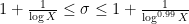 . However, from the Vinogradov-Korobov estimates (Exercise 43 of Notes 2) we have
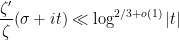
whenever  ; since we are assuming
  , the claim follows.
Exercise 20 Assume the Riemann hypothesis. Establish a bound of the form
for some absolute constant whenever  for a sufficiently large absolute constant . (Hint: use Perron’s formula and shift the contour to within
  of the critical line.) Use this to conclude that the upper bound
  in Proposition 19 can be relaxed (assuming RH) to
  .
.
Exercise 21 Let be a -bounded multiplicative function with  for all . For any , show that
Thus some sort of upper bound on in Proposition 19 is necessary.
Exercise 22 Let be a non-principal character of modulus  , and let be sufficiently large depending on . Show that

for all  . (One will need to adapt the Vinogradov-Korobov theory to Dirichet
  -functions.)
Proposition 19 measures how close the function lies to the Archimedean characters . Using the triangle inequality, one can then lower bound the distance of any other -bounded multiplicative function to these characters:
Proposition 23 Let be sufficiently large. Then for any -bounded multiplicative function , there exists a real number  with
with  such that

whenever  . In particular we have

if and  . If is real-valued, one can take
  .
.
Proof: For the first claim, choose to minimize  among all real numbers with . Then for any other , we see from the triangle inequality that

But from Proposition 19 we have


giving the first claim. When is real valued, we can similarly use the triangle inequality to bound


which gives

giving the second claim.
We can now quantify the non-pretentious nature of the Möbius and Liouville functions.
Exercise 24
— 2. Halasz’s inequality —
We now prove Halasz’s inequality. As a warm up, we prove Proposition 6:
Proof: (Proof of Proposition 6) By Exercise 16(iv) we may normalise  . We may assume that when , since the value of on these primes has no impact on the sum
  or on
or on  . In particular, from Euler products we now have the absolute convergence
  . Let
. Let  be a small quantity to be optimized later, and be smooth compactly supported function on
 ![{[-1,1]}](https://s0.wp.com/latex.php?latex=%7B%5B-1%2C1%5D%7D&bg=ffffff&fg=000000&s=0&c=20201002) that equals one on
that equals one on ![{[-1+\varepsilon,1+\varepsilon]}](https://s0.wp.com/latex.php?latex=%7B%5B-1%2B%5Cvarepsilon%2C1%2B%5Cvarepsilon%5D%7D&bg=ffffff&fg=000000&s=0&c=20201002) with the derivative bounds
with the derivative bounds  , on
, on ![{[-1,1] \backslash [-1+\varepsilon,1+\varepsilon]}](https://s0.wp.com/latex.php?latex=%7B%5B-1%2C1%5D+%5Cbackslash+%5B-1%2B%5Cvarepsilon%2C1%2B%5Cvarepsilon%5D%7D&bg=ffffff&fg=000000&s=0&c=20201002) , so on integration by parts we see that the Fourier transform
, so on integration by parts we see that the Fourier transform  obeys the bounds
for any and  . From the triangle inequality have

Applying Proposition 10 applied to a finite truncation of , and then using the absolute convergence of  and dominated convergence to eliminate the truncation (or by using Proposition 7 of Notes 2 and then shifting the contour), we can write the right-hand side as

which after rescaling by gives

Now from Lemma 18 one has


where  , and thus we can bound (12) by


if is chosen to be a sufficiently large absolute constant. The claim then follows by optimising in  .
.
We remark that an elementary proof of Proposition 6 with  was given in Proposition 1.2.6 of this monograph of Granville and Soundararajan. Also, in this paper of Lanzouri and Mangerel the variant estimate

is proven for any  . (Thanks to Andrew Granville for these references.)
It was observed by Granville, Koukoulopoulos, and Matomaki that we can also sharpen Proposition 6 when is non-negative by purely elementary methods:
Proposition 25 Let , and suppose that ![{f: {\bf N} \rightarrow [0,1]}](https://s0.wp.com/latex.php?latex=%7Bf%3A+%7B%5Cbf+N%7D+%5Crightarrow+%5B0%2C1%5D%7D&bg=ffffff&fg=000000&s=0&c=20201002) is multiplicative, -bounded, and non-negative. Then
is multiplicative, -bounded, and non-negative. Then

Proof: From Definition 5 and Mertens’ theorems the estimate is equivalent to

For the upper bound, we may assume that  vanishes for since these primes make no contribution to either side. We can then bound


For the lower bound, we let be the -bounded multiplicative function with  and
and  for and all primes . Then we observe the pointwise bound
  for all , hence
By the upper bound just obtained and Mertens’ theorems, we have
and the claim follows.
Now we can prove Theorem 7.
Proof: (Proof of Theorem 7) We may assume that  , since the claim is trivial otherwise. On the other hand, for
  for a sufficiently large , the second term on the right-hand side is dominated by the first, so the estimate does not become any stronger as one increases
  beyond
  , and hence we may assume without loss of generality that
  .
.
We abbreviate  , thus we wish to show that

It is convenient to remove some exceptional values of . Let  be a small quantity to be chosen later, subject to the restriction

From standard sieves (e.g., Theorem 32 from Notes 4), we see that the proportion of numbers in ![{[X/2,X]}](https://s0.wp.com/latex.php?latex=%7B%5BX%2F2%2CX%5D%7D&bg=ffffff&fg=000000&s=0&c=20201002) that do not have a “large” prime factor in
that do not have a “large” prime factor in ![{[X^\varepsilon,X]}](https://s0.wp.com/latex.php?latex=%7B%5BX%5E%5Cvarepsilon%2CX%5D%7D&bg=ffffff&fg=000000&s=0&c=20201002) , or do not have a “medium” prime factor in
, or do not have a “medium” prime factor in  , is
, is  . Thus by paying an error of , we may restrict to numbers that have at least one “large” prime factor in and at least one “medium” prime factor in (and no prime factor larger than ). This is the same as replacing with the Dirichlet convolution
where  is the restriction of to numbers with all prime factors in the “small” range
  ,
,  is the restriction of to numbers in
 ![{[2,X]}](https://s0.wp.com/latex.php?latex=%7B%5B2%2CX%5D%7D&bg=ffffff&fg=000000&s=0&c=20201002) with all prime factors in the “medium” range , and
with all prime factors in the “medium” range , and  is the restriction of to numbers in with all prime factors in the “large” range . We can thus write
This we can write in turn as

where ![{\psi(u) := 1_{[-\infty, 0]} e^u}](https://s0.wp.com/latex.php?latex=%7B%5Cpsi%28u%29+%3A%3D+1_%7B%5B-%5Cinfty%2C+0%5D%7D+e%5Eu%7D&bg=ffffff&fg=000000&s=0&c=20201002) . It is not advantageous to immediately apply Proposition 10 due to the rough nature of (which is not even Schwartz). But if we let
. It is not advantageous to immediately apply Proposition 10 due to the rough nature of (which is not even Schwartz). But if we let  be a Schwartz function of total mass whose Fourier transform is supported on , and define the mollified function
then one easily checks that

which from the triangle inequality soon gives the bounds

Hence we may write
Now we apply Proposition 10 and the triangle inequality to bound this by

But we may factor
and we may rather crudely bound  , hence we have
![\displaystyle \frac{1}{X} \sum_{n \leq X} f(n) \ll \| \tilde f \|_{FL^1([-T,T])} + \varepsilon + \frac{1}{T}.](https://s0.wp.com/latex.php?latex=%5Cdisplaystyle+%5Cfrac%7B1%7D%7BX%7D+%5Csum_%7Bn+%5Cleq+X%7D+f%28n%29+%5Cll+%5C%7C+%5Ctilde+f+%5C%7C_%7BFL%5E1%28%5B-T%2CT%5D%29%7D+%2B+%5Cvarepsilon+%2B+%5Cfrac%7B1%7D%7BT%7D.&bg=ffffff&fg=000000&s=0&c=20201002)
Using the Hölder inequalities (5), (6) we have
![\displaystyle \| \tilde f \|_{FL^1([-T,T])} \leq \| f_1 \|_{FL^\infty([-T,T])} \| f_2 \|_{FL^2([-T,T])} \| f_3 \|_{FL^2([-T,T])}.](https://s0.wp.com/latex.php?latex=%5Cdisplaystyle+%5C%7C+%5Ctilde+f+%5C%7C_%7BFL%5E1%28%5B-T%2CT%5D%29%7D+%5Cleq+%5C%7C+f_1+%5C%7C_%7BFL%5E%5Cinfty%28%5B-T%2CT%5D%29%7D+%5C%7C+f_2+%5C%7C_%7BFL%5E2%28%5B-T%2CT%5D%29%7D+%5C%7C+f_3+%5C%7C_%7BFL%5E2%28%5B-T%2CT%5D%29%7D.&bg=ffffff&fg=000000&s=0&c=20201002)
From Exercise 14 we have
![\displaystyle \| f_2 \|_{FL^2([-T,T])}^2 \ll \sum_n \frac{1}{n} (\frac{T}{n} \sum_{m: |n-m| \leq n/T} |f_2(m)|)^2.](https://s0.wp.com/latex.php?latex=%5Cdisplaystyle+%5C%7C+f_2+%5C%7C_%7BFL%5E2%28%5B-T%2CT%5D%29%7D%5E2+%5Cll+%5Csum_n+%5Cfrac%7B1%7D%7Bn%7D+%28%5Cfrac%7BT%7D%7Bn%7D+%5Csum_%7Bm%3A+%7Cn-m%7C+%5Cleq+n%2FT%7D+%7Cf_2%28m%29%7C%29%5E2.&bg=ffffff&fg=000000&s=0&c=20201002)
Note that is supported on ![{[X^{\varepsilon^2}, X]}](https://s0.wp.com/latex.php?latex=%7B%5BX%5E%7B%5Cvarepsilon%5E2%7D%2C+X%5D%7D&bg=ffffff&fg=000000&s=0&c=20201002) and hence is effectively also restricted to the range
and hence is effectively also restricted to the range  . From standard sieves (using (15)), we have

and thus
![\displaystyle \| f_2 \|_{FL^2([-T,T])}^2 \ll \frac{\varepsilon^{-O(1)}}{\log X}.](https://s0.wp.com/latex.php?latex=%5Cdisplaystyle+%5C%7C+f_2+%5C%7C_%7BFL%5E2%28%5B-T%2CT%5D%29%7D%5E2+%5Cll+%5Cfrac%7B%5Cvarepsilon%5E%7B-O%281%29%7D%7D%7B%5Clog+X%7D.&bg=ffffff&fg=000000&s=0&c=20201002)
Similarly
![\displaystyle \| f_3 \|_{FL^2([-T,T])}^2 \ll \frac{\varepsilon^{-O(1)}}{\log X}.](https://s0.wp.com/latex.php?latex=%5Cdisplaystyle+%5C%7C+f_3+%5C%7C_%7BFL%5E2%28%5B-T%2CT%5D%29%7D%5E2+%5Cll+%5Cfrac%7B%5Cvarepsilon%5E%7B-O%281%29%7D%7D%7B%5Clog+X%7D.&bg=ffffff&fg=000000&s=0&c=20201002)
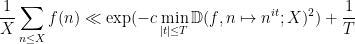
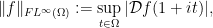
Finally, from Lemma 18 one has
![\displaystyle \| f_1 \|_{FL^\infty([-T,T])} \ll \log X^{\varepsilon^2} \exp( - \inf_{|t| \leq T} \mathbb{D}( f, n \mapsto n^{-it}; X^{\varepsilon^2})^2 )](https://s0.wp.com/latex.php?latex=%5Cdisplaystyle+%5C%7C+f_1+%5C%7C_%7BFL%5E%5Cinfty%28%5B-T%2CT%5D%29%7D+%5Cll+%5Clog+X%5E%7B%5Cvarepsilon%5E2%7D+%5Cexp%28+-+%5Cinf_%7B%7Ct%7C+%5Cleq+T%7D+%5Cmathbb%7BD%7D%28+f%2C+n+%5Cmapsto+n%5E%7B-it%7D%3B+X%5E%7B%5Cvarepsilon%5E2%7D%29%5E2+%29&bg=ffffff&fg=000000&s=0&c=20201002)


Putting all this together, we conclude that

Setting  for some sufficiently small constant (which in particular will ensure (15) since
  ), we obtain the claim.
One can optimise this argument to make the constant in Theorem 7 arbitrarily close to  ; see this previous post. With an even more refined argument, one can prove the sharper estimate
with  , a result initially due to Montgomery and Tenenbaum; see Theorem 2.3.1 of this text of Granville and Soundararajan. In the case of non-negative , an elementary argument gives the stronger bound
  ; see Corollary 1.2.3 of . However, the slightly weaker estimates in Theorem \ref Let be sufficiently large. Then for any real-valued -bounded multiplicative function , one has
for an absolute constant .
Thus for instance, setting  , we can use Wirsing’s theorem and Exercise 24 (or Mertens’ theorem) to recover a form of the prime number theorem with a modestly decaying error term, in that

for all large and some absolute constant . (Admittedly, we did use the far stronger Vinogradov-Korobov estimates earlier in this set of notes; but a careful inspection reveals that those estimates were not used in the proof of (16), so this is a non-circular proof of the prime number theorem.)
— 3. The Matomaki-Radziwill theorem —
We now give the proof of the Matomaki-Radziwill theorem, though we will leave several of the details to exercises. We first make a small but convenient reduction:
Exercise 26 Show that to prove Theorem 8, it suffices to do so for functions that are completely multiplicative. (This is similar to Exercise 1.)
Now we use Exercise 11 to phrase the theorem in an equivalent Fourier form:
Theorem 27 (Matomaki-Radziwill theorem, Fourier form) Let , and let  , with
  sufficiently large depending on . Let
  be a fixed smooth compactly supported function, and set
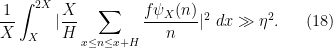
  . Suppose that is a -bounded completely multiplicative function such that
![\displaystyle \| f \psi_X \|_{FL^2([-T,T])} \gg \eta. \ \ \ \ \ (17)](https://s0.wp.com/latex.php?latex=%5Cdisplaystyle+%5C%7C+f+%5Cpsi_X+%5C%7C_%7BFL%5E2%28%5B-T%2CT%5D%29%7D+%5Cgg+%5Ceta.+%5C+%5C+%5C+%5C+%5C+%2817%29&bg=ffffff&fg=000000&s=0&c=20201002)
Then one has
for some  .
.
Let us assume Theorem 27 for the moment and see how it implies Theorem 8. In the latter theorem we may assume without loss of generality that is small. We may assume that  , since the case
 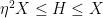 follows easily from Theorem \reF{halasz}.
Let be a smooth compactly supported function with  on
on ![{[-10,10]}](https://s0.wp.com/latex.php?latex=%7B%5B-10%2C10%5D%7D&bg=ffffff&fg=000000&s=0&c=20201002) . By hypothesis, we have
. By hypothesis, we have
Let be a Schwartz function of mean whose Fourier transform is supported on . For any ![{x\in [X,2X]}](https://s0.wp.com/latex.php?latex=%7Bx%5Cin+%5BX%2C2X%5D%7D&bg=ffffff&fg=000000&s=0&c=20201002) , we consider the expression
, we consider the expression
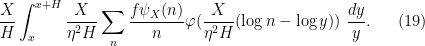
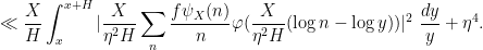
A routine calculation using the rapid decrease of shows that
![\displaystyle \frac{X}{\eta^2 H} \int_x^{x+H} \varphi( \frac{X}{\eta^2 H} (\log n - \log y) )\ \frac{dy}{y} = 1_{[x,x+H]}(n)](https://s0.wp.com/latex.php?latex=%5Cdisplaystyle+%5Cfrac%7BX%7D%7B%5Ceta%5E2+H%7D+%5Cint_x%5E%7Bx%2BH%7D+%5Cvarphi%28+%5Cfrac%7BX%7D%7B%5Ceta%5E2+H%7D+%28%5Clog+n+-+%5Clog+y%29+%29%5C+%5Cfrac%7Bdy%7D%7By%7D+%3D+1_%7B%5Bx%2Cx%2BH%5D%7D%28n%29+&bg=ffffff&fg=000000&s=0&c=20201002)

and thus the expression (19) can be estimated as
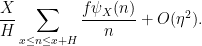
By Cauchy-Schwarz we then have

Averaging this for ![{x \in [X,2X]}](https://s0.wp.com/latex.php?latex=%7Bx+%5Cin+%5BX%2C2X%5D%7D&bg=ffffff&fg=000000&s=0&c=20201002) and using Fubini’s theorem, we have
and using Fubini’s theorem, we have

and thus from (18) and the triangle inequality we have
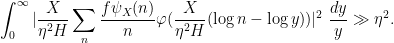
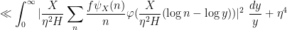
On the other hand, from Exercise 11 we have
![\displaystyle \int_0^\infty |\frac{X}{\eta^2 H} \sum_n \frac{f\psi_X(n)}{n} \varphi( \frac{X}{\eta^2 H} (\log n - \log y) )|^2\ \frac{dy}{y} \ll \| f \psi_X \|_{FL^2([-T,T])}^2.](https://s0.wp.com/latex.php?latex=%5Cdisplaystyle+%5Cint_0%5E%5Cinfty+%7C%5Cfrac%7BX%7D%7B%5Ceta%5E2+H%7D+%5Csum_n+%5Cfrac%7Bf%5Cpsi_X%28n%29%7D%7Bn%7D+%5Cvarphi%28+%5Cfrac%7BX%7D%7B%5Ceta%5E2+H%7D+%28%5Clog+n+-+%5Clog+y%29+%29%7C%5E2%5C+%5Cfrac%7Bdy%7D%7By%7D+%5Cll+%5C%7C+f+%5Cpsi_X+%5C%7C_%7BFL%5E2%28%5B-T%2CT%5D%29%7D%5E2.&bg=ffffff&fg=000000&s=0&c=20201002)
Applying Theorem 27 (with a slightly smaller value of and ), we obtain the claim.
Exercise 28 In the converse direction, show that Theorem 27 is a consequence of Theorem 8.
Exercise 29 Let be supported on ![{[X,3X]}](https://s0.wp.com/latex.php?latex=%7B%5BX%2C3X%5D%7D&bg=ffffff&fg=000000&s=0&c=20201002) , and let . Show that
, and let . Show that


(Hint: use summation by parts to express  as a suitable linear combination of sums
  and
and  , then use the Cauchy-Schwarz inequality and the Fubini-Tonelli theorem.) Conclude in particular that


where  . (This argument is due to Saffari and Vaughan.)
It remains to establish Theorem 27. As before we may assume that is small. Let us call a finitely supported arithmetic function large on some subset of ![{[-X,X]}](https://s0.wp.com/latex.php?latex=%7B%5B-X%2CX%5D%7D&bg=ffffff&fg=000000&s=0&c=20201002) if
if

and small on if
Note that a function cannot be simultaneously large and small on the same set ; and if a function is large on some subset , then it remains large on after modifying by any small error (assuming is small enough, and adjusting the implied constants appropriately). From the hypothesis (17) we know that  is large on . As discussed in the introduction, the strategy is now to decompose into various regions, and on each of these regions split (up to small errors) as an average of Dirichlet convolutions of other factors which enjoy either good estimates or good estimates on the given region.
We will need the following ranges:
We will be able to cover the range  just using arguments involving the zeroth interval
 ![{[P_0,Q_0]}](https://s0.wp.com/latex.php?latex=%7B%5BP_0%2CQ_0%5D%7D&bg=ffffff&fg=000000&s=0&c=20201002) ; the range
; the range  can be covered using arguments involving the zeroth interval and the first interval
 ![{[P_1,Q_1]}](https://s0.wp.com/latex.php?latex=%7B%5BP_1%2CQ_1%5D%7D&bg=ffffff&fg=000000&s=0&c=20201002) ; and the range
; and the range  can be covered using arguments involving all three intervals
 ![{[P_0,Q_0], [P_1,Q_1], [P_2,Q_2]}](https://s0.wp.com/latex.php?latex=%7B%5BP_0%2CQ_0%5D%2C+%5BP_1%2CQ_1%5D%2C+%5BP_2%2CQ_2%5D%7D&bg=ffffff&fg=000000&s=0&c=20201002) . Coverage of the remaining ranges of can be done by an extension of the methods given here and will be left to the exercises at the end of the notes.
. Coverage of the remaining ranges of can be done by an extension of the methods given here and will be left to the exercises at the end of the notes.
We introduce some weight functions and some exceptional sets. For any  , let
, let  be a bump function on of total mass , and let
  denote the arithmetic function
supported on the primes  . We then define the following subsets of :
We will establish the following claims:
Proposition 30
- (i) If
 for some
  , then is small on
 ![{[-T,T] \backslash \Omega_i}](https://s0.wp.com/latex.php?latex=%7B%5B-T%2CT%5D+%5Cbackslash+%5COmega_i%7D&bg=ffffff&fg=000000&s=0&c=20201002) .
.
- (ii) is small on
 .
.
- (iii) is small on
 .
.
- (iv) If is large on
![{[-T,T] \cap \Omega_0}](https://s0.wp.com/latex.php?latex=%7B%5B-T%2CT%5D+%5Ccap+%5COmega_0%7D&bg=ffffff&fg=000000&s=0&c=20201002) , then one has
, then one has  for some .
Note that parts (i) (with  ) and (iv) of the claims are already enough to treat the case ; parts (i) (with
  ), (ii), and (iv) are enough to treat the case ; and parts (i) (with
  ), (ii), (iii), and (iv) are enough to treat the case .
We first prove (i). For , let ![{\tilde w_{[P_i,Q_i]}}](https://s0.wp.com/latex.php?latex=%7B%5Ctilde+w_%7B%5BP_i%2CQ_i%5D%7D%7D&bg=ffffff&fg=000000&s=0&c=20201002) denote the function
denote the function
![\displaystyle \tilde w_{[P_i,Q_i]} := \frac{1}{\log \frac{\log Q_i}{\log P_i}} \sum_{P \in [P_i,Q_i]} \frac{1}{\log P} w_P. \ \ \ \ \ (20)](https://s0.wp.com/latex.php?latex=%5Cdisplaystyle+%5Ctilde+w_%7B%5BP_i%2CQ_i%5D%7D+%3A%3D+%5Cfrac%7B1%7D%7B%5Clog+%5Cfrac%7B%5Clog+Q_i%7D%7B%5Clog+P_i%7D%7D+%5Csum_%7BP+%5Cin+%5BP_i%2CQ_i%5D%7D+%5Cfrac%7B1%7D%7B%5Clog+P%7D+w_P.+%5C+%5C+%5C+%5C+%5C+%2820%29&bg=ffffff&fg=000000&s=0&c=20201002)
This function is a variant of the function ![{w_{[P_i,Q_i]}}](https://s0.wp.com/latex.php?latex=%7Bw_%7B%5BP_i%2CQ_i%5D%7D%7D&bg=ffffff&fg=000000&s=0&c=20201002) introduced in (7). A key point is that the convolutions
introduced in (7). A key point is that the convolutions ![{1 * w_{[P_i,Q_i]}}](https://s0.wp.com/latex.php?latex=%7B1+%2A+w_%7B%5BP_i%2CQ_i%5D%7D%7D&bg=ffffff&fg=000000&s=0&c=20201002) stay close to :
stay close to :
Exercise 31 (Turan-Kubilius inequalities) For , show that
![\displaystyle \frac{1}{X} \sum_{X/2 \leq n \leq 4X} |1*\tilde w_{[P_i,Q_i]}(n) - 1|^2 \ll \eta^4.](https://s0.wp.com/latex.php?latex=%5Cdisplaystyle+%5Cfrac%7B1%7D%7BX%7D+%5Csum_%7BX%2F2+%5Cleq+n+%5Cleq+4X%7D+%7C1%2A%5Ctilde+w_%7B%5BP_i%2CQ_i%5D%7D%28n%29+-+1%7C%5E2+%5Cll+%5Ceta%5E4.&bg=ffffff&fg=000000&s=0&c=20201002)
(Hint: use the second moment method, as in the proof of Lemma 2 of Notes 9.)
Let . Inserting the bounded factor  in the above estimates, and applying Exercise 14, we conclude in particular that the expression
![\displaystyle f \psi_X (1 * \tilde w_{[P_i,Q_i]}) - f \psi_X](https://s0.wp.com/latex.php?latex=%5Cdisplaystyle+f+%5Cpsi_X+%281+%2A+%5Ctilde+w_%7B%5BP_i%2CQ_i%5D%7D%29+-+f+%5Cpsi_X&bg=ffffff&fg=000000&s=0&c=20201002)
is small on . Since is completely multiplicative, we can write this expression as
![\displaystyle (f * (f\tilde w_{[P_i,Q_i]})) \psi_X - f \psi_X](https://s0.wp.com/latex.php?latex=%5Cdisplaystyle+%28f+%2A+%28f%5Ctilde+w_%7B%5BP_i%2CQ_i%5D%7D%29%29+%5Cpsi_X+-+f+%5Cpsi_X+&bg=ffffff&fg=000000&s=0&c=20201002)
We now perform some technical manipulations to move the cutoff  to a more convenient location. From (20) we have
![\displaystyle (f * (f \tilde w_{[P_i,Q_i]})) \psi_X = \frac{1}{\log\frac{\log Q_i}{\log P_i}} \sum_{P \in [P_i,Q_i]} \frac{1}{\log P} (f * (f w_{P})) \psi_X.](https://s0.wp.com/latex.php?latex=%5Cdisplaystyle+%28f+%2A+%28f+%5Ctilde+w_%7B%5BP_i%2CQ_i%5D%7D%29%29+%5Cpsi_X+%3D+%5Cfrac%7B1%7D%7B%5Clog%5Cfrac%7B%5Clog+Q_i%7D%7B%5Clog+P_i%7D%7D+%5Csum_%7BP+%5Cin+%5BP_i%2CQ_i%5D%7D+%5Cfrac%7B1%7D%7B%5Clog+P%7D+%28f+%2A+%28f+w_%7BP%7D%29%29+%5Cpsi_X.&bg=ffffff&fg=000000&s=0&c=20201002)
We would like to approximate  by
by  . A brief triangle inequality calculation using the smoothness of , the -boundedness of , and the narrow support of
  shows that

where  is defined similarly to but with a slightly larger choice of initial cutoff
  . Integrating this we conclude that
![\displaystyle (f * (f \tilde w_{[P_i,Q_i]})) \psi_X](https://s0.wp.com/latex.php?latex=%5Cdisplaystyle+%28f+%2A+%28f+%5Ctilde+w_%7B%5BP_i%2CQ_i%5D%7D%29%29+%5Cpsi_X&bg=ffffff&fg=000000&s=0&c=20201002)
![\displaystyle = \frac{1}{\log\frac{\log Q_i}{\log P_i}} \sum_{P \in [P_i,Q_i]} \frac{1}{\log P} ((f\psi_{X/P}) * (f w_{P}))](https://s0.wp.com/latex.php?latex=%5Cdisplaystyle+%3D+%5Cfrac%7B1%7D%7B%5Clog%5Cfrac%7B%5Clog+Q_i%7D%7B%5Clog+P_i%7D%7D+%5Csum_%7BP+%5Cin+%5BP_i%2CQ_i%5D%7D+%5Cfrac%7B1%7D%7B%5Clog+P%7D+%28%28f%5Cpsi_%7BX%2FP%7D%29+%2A+%28f+w_%7BP%7D%29%29&bg=ffffff&fg=000000&s=0&c=20201002)
![\displaystyle + O( \eta^4 (1 * \tilde w_{[P_i,Q_i]}) \tilde \psi_X ).](https://s0.wp.com/latex.php?latex=%5Cdisplaystyle+%2B+O%28+%5Ceta%5E4+%281+%2A+%5Ctilde+w_%7B%5BP_i%2CQ_i%5D%7D%29+%5Ctilde+%5Cpsi_X+%29.&bg=ffffff&fg=000000&s=0&c=20201002)
Using Exercise 31 and Exercise 14, the error term is small on . Thus we conclude that
![\displaystyle \frac{1}{\log\frac{\log Q_i}{\log P_i}} \sum_{P \in [P_i,Q_i]} \frac{1}{\log P_i} ((f\psi_{X/P}) * (f w_{P})) - f \psi_X \ \ \ \ \ (21)](https://s0.wp.com/latex.php?latex=%5Cdisplaystyle+%5Cfrac%7B1%7D%7B%5Clog%5Cfrac%7B%5Clog+Q_i%7D%7B%5Clog+P_i%7D%7D+%5Csum_%7BP+%5Cin+%5BP_i%2CQ_i%5D%7D+%5Cfrac%7B1%7D%7B%5Clog+P_i%7D+%28%28f%5Cpsi_%7BX%2FP%7D%29+%2A+%28f+w_%7BP%7D%29%29+-+f+%5Cpsi_X+%5C+%5C+%5C+%5C+%5C+%2821%29&bg=ffffff&fg=000000&s=0&c=20201002)
is small on , and hence also on . Thus by the triangle inequality, it will suffice to show that

is small on for each ![{P \in [P_i,Q_i]}](https://s0.wp.com/latex.php?latex=%7BP+%5Cin+%5BP_i%2CQ_i%5D%7D&bg=ffffff&fg=000000&s=0&c=20201002) . But by construction we definitely have
. But by construction we definitely have
![\displaystyle \|fw_P \|_{FL^\infty([-T,T] \backslash \Omega_i)} \ll \eta^4](https://s0.wp.com/latex.php?latex=%5Cdisplaystyle+%5C%7Cfw_P+%5C%7C_%7BFL%5E%5Cinfty%28%5B-T%2CT%5D+%5Cbackslash+%5COmega_i%29%7D+%5Cll+%5Ceta%5E4&bg=ffffff&fg=000000&s=0&c=20201002)
while from Exercise 14 and the hypothesis  we have
![\displaystyle \|f \psi_{X/P} \|_{FL^2([-T,T] \backslash \Omega_i)} \ll 1](https://s0.wp.com/latex.php?latex=%5Cdisplaystyle+%5C%7Cf+%5Cpsi_%7BX%2FP%7D+%5C%7C_%7BFL%5E2%28%5B-T%2CT%5D+%5Cbackslash+%5COmega_i%29%7D+%5Cll+1&bg=ffffff&fg=000000&s=0&c=20201002)
and the claim (i) now follows from (6).
We now jump to (iv). The first observation is that the set  is quite small. To quantify this we use the following bound:
Proposition 32 (Large values of  ) Let be sufficiently large depending on , and let
  . Then for any
  , the set
![\displaystyle \Omega := \{ t \in [-X,X]: |{\mathcal D} w_P(1+it)| \geq \sigma \}](https://s0.wp.com/latex.php?latex=%5Cdisplaystyle+%5COmega+%3A%3D+%5C%7B+t+%5Cin+%5B-X%2CX%5D%3A+%7C%7B%5Cmathcal+D%7D+w_P%281%2Bit%29%7C+%5Cgeq+%5Csigma+%5C%7D&bg=ffffff&fg=000000&s=0&c=20201002)
has measure at most  .
.
Proof: We use the high moment method. Let  be a natural number to be optimised in later, and let
  be the convolution of copies of . Then on we have
  . Thus by Markov’s inequality, the measure of is at most
![\displaystyle \sigma^{-2k} \| w_P^{*k} \|_{FL^2([-X,X])}^2.](https://s0.wp.com/latex.php?latex=%5Cdisplaystyle+%5Csigma%5E%7B-2k%7D+%5C%7C+w_P%5E%7B%2Ak%7D+%5C%7C_%7BFL%5E2%28%5B-X%2CX%5D%29%7D%5E2.&bg=ffffff&fg=000000&s=0&c=20201002)
To bound this we use Exercise 14. If we choose to be the first integer for which  , then this exercise gives us the bound
![\displaystyle \| w_P^{*k} \|_{FL^2([-X,X])}^2 \ll O_\eta(1)^{O(k)} \frac{1}{P^k} \sum_n w_P^{*k}(n)^2.](https://s0.wp.com/latex.php?latex=%5Cdisplaystyle+%5C%7C+w_P%5E%7B%2Ak%7D+%5C%7C_%7BFL%5E2%28%5B-X%2CX%5D%29%7D%5E2+%5Cll+O_%5Ceta%281%29%5E%7BO%28k%29%7D+%5Cfrac%7B1%7D%7BP%5Ek%7D+%5Csum_n+w_P%5E%7B%2Ak%7D%28n%29%5E2.&bg=ffffff&fg=000000&s=0&c=20201002)
From the fundamental theorem of arithmetic we see that  , hence
From the prime number theorem we have  . Putting all this together, we conclude that the measure of is at most

Since  , we obtain the claim.
Applying this proposition with  ranging between
  and
and  and
and  , and applying the union bound, the we see that the measure of is at most
  . To exploit this, we will need some bounds of Vinogradov-Korobov type:
Exercise 33 (Vinogradov bounds) For  , establish the bound


for any and . (Hint: replace with a weighted version of the von Mangoldt function, apply Proposition 7 of Notes 2, and shift the contour, using the zero free region from Exercise 43 of Notes 2.)
Now we can establish we use the following variant of the Montgomery-Halasz large values theorem (cf. Proposition 9 from Notes 6):
Proposition 34 (Montgomery-Halasz for primes) Let , let ![{P \in [P_0,Q_0]}](https://s0.wp.com/latex.php?latex=%7BP+%5Cin+%5BP_0%2CQ_0%5D%7D&bg=ffffff&fg=000000&s=0&c=20201002) , and
, and ![{\Omega \subset [-X,X]}](https://s0.wp.com/latex.php?latex=%7B%5COmega+%5Csubset+%5B-X%2CX%5D%7D&bg=ffffff&fg=000000&s=0&c=20201002) have measure
have measure  . Then for any -bounded function , one has

Proof: By duality, we may write
for some measurable function  with
with  . We can rearrange the right-hand side as

which by Cauchy-Schwarz is boudned in magnitude by

We can rearrange this as

which by the elementary inequality  is bounded by

(cf. Lemma 6 from Notes 9). By Exercise 33 we have

The claim follows.
Now we can prove (iv). By hypothesis,  is large on . On the other hand, the function (21) (with ) is small on . By the triangle inequality, we conclude that
![\displaystyle \frac{1}{\log\frac{\log Q_0}{\log P_0}} \sum_{P \in [P_0,Q_0]} \frac{1}{\log P_0} ((f\psi_{X/P}) * (f w_{P}))](https://s0.wp.com/latex.php?latex=%5Cdisplaystyle+%5Cfrac%7B1%7D%7B%5Clog%5Cfrac%7B%5Clog+Q_0%7D%7B%5Clog+P_0%7D%7D+%5Csum_%7BP+%5Cin+%5BP_0%2CQ_0%5D%7D+%5Cfrac%7B1%7D%7B%5Clog+P_0%7D+%28%28f%5Cpsi_%7BX%2FP%7D%29+%2A+%28f+w_%7BP%7D%29%29+&bg=ffffff&fg=000000&s=0&c=20201002)
is large on , hence by the pigeonhole principle, there exists such that
is large on . On the other hand, from Proposition 32 and Prosition 34 we have
![\displaystyle \| f w_P \|_{FL^2([-T,T] \cap \Omega_0)} \ll_{\eta} 1,](https://s0.wp.com/latex.php?latex=%5Cdisplaystyle+%5C%7C+f+w_P+%5C%7C_%7BFL%5E2%28%5B-T%2CT%5D+%5Ccap+%5COmega_0%29%7D+%5Cll_%7B%5Ceta%7D+1%2C&bg=ffffff&fg=000000&s=0&c=20201002)
hence by (6)
![\displaystyle \| f\psi_{X/P} \|_{FL^\infty([-T,T] \cap \Omega_0)} \gg_\eta 1.](https://s0.wp.com/latex.php?latex=%5Cdisplaystyle+%5C%7C+f%5Cpsi_%7BX%2FP%7D+%5C%7C_%7BFL%5E%5Cinfty%28%5B-T%2CT%5D+%5Ccap+%5COmega_0%29%7D+%5Cgg_%5Ceta+1.&bg=ffffff&fg=000000&s=0&c=20201002)
By the pigeonhole principle, this implies that
![\displaystyle \| f 1_I \|_{FL^\infty([-T,T] \cap \Omega_0)} \gg_\eta 1.](https://s0.wp.com/latex.php?latex=%5Cdisplaystyle+%5C%7C+f+1_I+%5C%7C_%7BFL%5E%5Cinfty%28%5B-T%2CT%5D+%5Ccap+%5COmega_0%29%7D+%5Cgg_%5Ceta+1.&bg=ffffff&fg=000000&s=0&c=20201002)
for some interval ![{I \subset [X/10P, 10X/P]}](https://s0.wp.com/latex.php?latex=%7BI+%5Csubset+%5BX%2F10P%2C+10X%2FP%5D%7D&bg=ffffff&fg=000000&s=0&c=20201002) . The claim (iv) now follows from Exercise 13. Note that this already concludes the argument in the range
. The claim (iv) now follows from Exercise 13. Note that this already concludes the argument in the range  .
.
Now we establish (ii). Here the set  is not as well controlled in size as , but is still quite small. Indeed, from applying Proposition 32 with ranging between
  and
and  and
and  , and applying the union bound, the we see that the measure of is at most
  . This is too large of a bound to apply Proposition 34, but we may instead apply a different bound:
Exercise 35 (Montgomery-Halasz for integers) Let , and let have measure  . For any -bounded function supported on
 ![{[X^{0.8},2X]}](https://s0.wp.com/latex.php?latex=%7B%5BX%5E%7B0.8%7D%2C2X%5D%7D&bg=ffffff&fg=000000&s=0&c=20201002) , show that
, show that
(It is possible to remove the logarithmic loss here by being careful, but this loss will be acceptable for our arguments. One can either repeat the arguments used to prove Proposition 34, or else appeal to Proposition 9 from Notes 6.)
The point here is that we can get good bounds even when the function is supported at narrower scales (such as  ) than the Fourier interval under consideration (such as or ). In particular, this exercise will serve as a replacement for Exercise 14, which will not give good estimates in this case.
As before, the function (21) is small on , so it will suffice by the triangle inequality to show that
is small on for all . From Exercise 35, we have

while from definition of we have
and the claim now follows from (6). Note that this already concludes the argument in the range .
Finally, we establish (iii). The function (21) (with ) is small on , so by the triangle inequality as before it suffices to show that
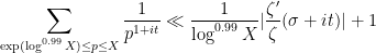
is small on for all ![{P \in [P_1,Q_1]}](https://s0.wp.com/latex.php?latex=%7BP+%5Cin+%5BP_1%2CQ_1%5D%7D&bg=ffffff&fg=000000&s=0&c=20201002) . On the one hand, the definition of gives a good bound on
. On the one hand, the definition of gives a good bound on  :
:

To conclude using (6) we now need a good bound for  . Unfortunately, the function
  is now supported on too short of an interval for Exercise 14 to give good estimates, and
  is too large for Exercise 35 to be applicable either.
But from definition we see that for  , we have

for at least one ![{P' \in [P_2,Q_2]}](https://s0.wp.com/latex.php?latex=%7BP%27+%5Cin+%5BP_2%2CQ_2%5D%7D&bg=ffffff&fg=000000&s=0&c=20201002) . We can use this to amplify the power of Exercise 14:
. We can use this to amplify the power of Exercise 14:
Proposition 36 (Amplified mean value estimate) One has  .
.
Proof: For each , let  denote the set of
 ![{t \in [-X,X]}](https://s0.wp.com/latex.php?latex=%7Bt+%5Cin+%5B-X%2CX%5D%7D&bg=ffffff&fg=000000&s=0&c=20201002) where (23) holds. Since there are
where (23) holds. Since there are  values of
  , and
, and  , it suffices by the union bound to show that

(say) for each . Let be the first integer for which the quantity  , thus
From (23) we have the pointwise bound

and hence by Exercise 14

where  . As is -bounded, and the summand only vanishes when
  , we can bound the right-hand side by
where  denotes the set of primes in the interval
 ![{[P'/2, 2P']}](https://s0.wp.com/latex.php?latex=%7B%5BP%27%2F2%2C+2P%27%5D%7D&bg=ffffff&fg=000000&s=0&c=20201002) .
.
Suppose has  prime factors in this interval (counting multiplicity). Then
  vanishes unless
  , in which case we can bound
and

Thus we may bound the above sum by

By the prime number theorem, has  elements, so by double counting we have

and thus the previous bound becomes
which sums to
Since

we thus have


so that  , we obtain the claim.
Combining this proposition with (22) and (6), we conclude part (iii) of Proposition 30. This establishes Theorem 27 up to the range  .
.
Exercise 37 Show that for any fixed  , Theorem 27 holds in the range
where  denotes the -fold iterated logarithm of . (Hint: this is already accomplished for
  . For higher , one has to introduce additional exceptional intervals
  and extend Proposition 30 appropriately.)
Exercise 38 Establish Theorem 27 (and hence Theorem 8) in full generality. (This is the preceding exercise, but now with potentially as large as  , where the inverse tower exponential function
  is defined as the least for which
  . Now one has to start tracking dependence on of all the arguments in the above analysis; in particular, the convenient notation of arithmetic functions being “large” or “small” needs to be replaced with something more precise.)

.


would hold for almost all
for which
is extremely large.)
replaced by
, where
is the principal character of period
for all


, with equality if and only if
and
. (Hint: for the last property, apply Lemma 15 to a suitable Hilbert space
.
, then
,
and
for all
.


.


is the interval
![\displaystyle [P_0,Q_0] := [\exp( \log^{0.9} X ), \exp( \log^{0.95} X )].](https://s0.wp.com/latex.php?latex=%5Cdisplaystyle+%5BP_0%2CQ_0%5D+%3A%3D+%5B%5Cexp%28+%5Clog%5E%7B0.9%7D+X+%29%2C+%5Cexp%28+%5Clog%5E%7B0.95%7D+X+%29%5D.&bg=ffffff&fg=000000&s=0&c=20201002)
![\displaystyle [P_1,Q_1] := [\exp( (\log\log X)^2 ), \exp( (\log\log X)^3 )].](https://s0.wp.com/latex.php?latex=%5Cdisplaystyle+%5BP_1%2CQ_1%5D+%3A%3D+%5B%5Cexp%28+%28%5Clog%5Clog+X%29%5E2+%29%2C+%5Cexp%28+%28%5Clog%5Clog+X%29%5E3+%29%5D.&bg=ffffff&fg=000000&s=0&c=20201002)
![\displaystyle [P_2,Q_2] := [\exp( (\log\log\log X)^2 ), \exp( (\log\log\log X)^3 )].](https://s0.wp.com/latex.php?latex=%5Cdisplaystyle+%5BP_2%2CQ_2%5D+%3A%3D+%5B%5Cexp%28+%28%5Clog%5Clog%5Clog+X%29%5E2+%29%2C+%5Cexp%28+%28%5Clog%5Clog%5Clog+X%29%5E3+%29%5D.&bg=ffffff&fg=000000&s=0&c=20201002)
.


19 comments
Comments feed for this article
17 December, 2019 at 10:34 am
Anonymous
What is the current best value for the constant in proposition 6 ?
17 December, 2019 at 11:42 am
Terence Tao
For non-negative functions, the Granville-Koukoulopoulos-Matomaki result given as in Proposition 25 in this blog lets one take , so it is reasonable to conjecture at least that one can take
  in general (which would be broadly consistent with the situation with the non-logarithmically averaged Halasz conjecture, though in that case there is a lower order factor of
  that is necessarily lost). But I don’t know of a place where this appears in the literature. Perhaps one just has to refine the methods that are already present in this post to get the sharp constant.
18 December, 2019 at 9:46 am
Terence Tao
Actually, after doing some calculations it seems that the optimal constant should be strictly less than 1 if
  is not real. Basically, if one has
for all , then by summation by parts we should also have
which after taking logarithms (using Lemma 18, and assuming one of the technical conditions of that lemma) becomes
If we assume for
for  , this becomes
If one chooses to be a unit complex number canceling the phase of
  , then this implies (after using Mertens’ theorems) that
which is not true for (the LHS is
  and the RHS is
  ) so forces
  to be strictly less than 1 (I have not calculated the precise upper bound on
  this constraint forces). This may even provide the optimal value of
  , but I have not carefully checked this. However for
  real this argument does not seem to prevent
  , which is of course consistent with the Granville-Koukoulopolous-Matomaki result.
19 December, 2019 at 9:17 am
Terence Tao
After doing further calculations and also talking with Andrew Granville it does seem that the optimal exponent for complex-valued is indeed the unique real number
  solving the equation
(note the LHS is strictly increasing in ) and more precisely I can show the inequality
for any . The secondary error
  is due to the reliance on Vinogradov-Korobov type estimates and I think it can be deleted if one assumes RH. Thanks to Andrew for calculating
  and also pointing out that the
  case of the bound was established by elementary means in his book with Sound. The argument sketched in the previous comment shows that
  is optimal, though it is still possible that the epsilon loss could be removed or replaced with some explicit lower order term.
Sketch of proof: by smoothing out the sum on the LHS (as in the lecture notes, with replaced by
  ) the left-hand side can be bounded up to acceptable errors by
(assuming that for
for  , otherwise replace
  by
by  here) so by dyadic decomposition it suffices to show that
for every (the contribution of
  can be easily handled) and some
  depending only on
  . Using Lemma 18 this can be reduced as
The contributions of can be cancelled out without much difficulty using Mertens’ theorems, leaving one with
Using a Halasz type theorem for the primes in the regime one can show that
  for all
  outside of
  unit intervals. This gives an acceptable contribution outside of these intervals (because of the gap between
  and
and  ) so it remains to establish the pointwise bound

so on taking logarithms and using the triangle inequality it suffices to show that
But by the prime number theorem, and summation by parts the left-hand side is
and the claim now follows from the construction of .
.
In the case when is real, one replaces
  by
by  , and it seems the same argument now allows one to replace
  with
with  . I haven’t thought about whether the epsilon losses in the above argument can be removed in this case.
23 December, 2019 at 6:12 am
Smangerel
When is real-valued and 1-bounded the (unconditional) inequality you gave can be sharpened to
in particular with , at least when
  does not behave too much like the M\”{o}bius function.
 can be assumed completely multiplicative without changing the order of magnitude in logarithmic averages (this can be shown as follows: define
  to denote the completely multiplicative function defined on primes with
  then, writing
  ,
,  is supported on squarefulls. Then use the hyperbola method.).
 completely multiplicative, one easily sees that
  is non-negative and multiplicative, and moreover that
To see this, it is convenient first to observe that
With
and since is divisor bounded one can use e.g., Shiu’s theorem to establish that
as required. , one can improve the
  slightly, as is done in Proposition 3.1 of https://arxiv.org/pdf/math/0508361v1.pdf; to remove it entirely one would need to replace
  by
by  which seems quite hard.
By handling the term with fractional parts in the estimate for the mean value of
23 December, 2019 at 7:55 am
Terence Tao
Very slick! It’s nice to know that elementary methods are competitive with (and in this case, slightly superior to) the Fourier analytic/complex analytic methods sometimes :)
Andrew Granville also pointed out to me the bound
for any complex -bounded
  and
and  , established as Theorem 1.4 of your paper with Lamzouri. He suggested that the
  inequality could be deduced from this one, though I wasn’t able to see a direct way to do this.
17 December, 2019 at 10:02 pm
David Roberts
“…shown by Motohashi that one can also establish (4) as long as…”
that (4) links to (3), which I suspect the text should reflect.
[Corrected, thanks – T.]
24 December, 2019 at 9:53 am
Anonymous
In line 7, it seems that “multiplicative group ”
” ”
”
should be “additive group
[Actually, I do mean the multiplicative group here; the positive reals
  form a group under multiplication, but are merely a monoid under addition.)
30 July, 2020 at 7:12 pm
Higher uniformity of bounded multiplicative functions in short intervals on average | What's new
[…] which was proven (for arbitrarily slowly growing ) in a landmark paper of Matomäki and Radziwill, discussed for instance in this blog post. […]
12 October, 2020 at 1:28 pm
254A announcement: Analytic prime number theory | What's new
[…] Halasz’s theorem and the Matomaki-Radziwill theorem […]
3 May, 2022 at 9:08 am
Anonymous
In exercise 4, I think you might have the hints swapped. Sorry if I’m missing something obvious.
[Corrected, thanks – T.]
12 May, 2022 at 4:01 pm
Rory
Typo in the proof of Proposition 19: “Now suppose that .”
.”
[Corrected, thanks – T.]
16 May, 2022 at 12:31 pm
Anonymous
In Exercise 21, there seems to be a typo. You define a function which you do not use in the exercise itself.
[Corrected, thanks – T.]
13 November, 2022 at 2:12 am
Quân Nguyễn
Dear prof. Tao, .
.
On the left of “However, from the Vinogradov-Korobov”, I think it should be
[Corrected, thanks – T.]
In Exercise 20 the second part, if one assumes Riemann Hypothesis, then from the bound and the Log-truncated formula, one already obtains
  which is sufficient to establish the bound
  without the needs to use the first part of Exercise 20.
[I am afraid I do not see how to get a double logarithmic bound on , which would require
  to stay a distance
  away from any zeroes. -T]
27 November, 2022 at 7:20 am
Quân Nguyễn
Dear prof. Tao,
The function in the integrand in equation below “On the other hand, from Exercise 11 we have” should have been \varphi( \frac{X}{\eta^2 H} (\log n – \log y) )?
And in the RHS of the second equations of Exercise 29 should have been in terms of $$dt$$.
Also, I think the RHS of the first equation of Exercise 29, the factor before the integral should be 1/(H/X)? Cause If one tries with f(n) = 1 supported in [X, 3X] then the inequality turns out to be false.
Thank you for your time.
[Corrected, thanks – T.]
18 June, 2023 at 9:51 pm
Anonymous
FYI – there seems to be some issue with wordpress where the post that was previously here has been replaced with the most recent blog post for some reason, at least on my end.
[Corrected, thanks -T.]
14 July, 2023 at 5:12 pm
James
Is there a factor of missing from either the definition of
  or
or  (in Section 3 around where the bullet points are)? I’m not getting that the expectation of
  is roughly 1, and so Exercise 31 seems to not hold as currently written? However, if you introduce a factor of
  in
in  , then the expectation of
  does appear to be roughly
  .
.
[Corrected, thanks – T.]
17 July, 2023 at 1:58 pm
James
But if you put the $1/P$ in the definition of $w_P$, then I’m not sure that $(fw_P) * (f\psi_{X/P})$ is small implies that (21) is small. Should the $1/P$ go in the definition of $\tilde{w}$ instead of $w/P$ (so that you have a $\log\log$ average)?
19 July, 2023 at 2:53 pm
James
In the proof of Proposition 32, why is it true that $w^{*k}_P(n) \ll k^k$? I’m getting that $w^{*k}_P(n) \ll k! \frac{\log(P)^k}{\eta^{4k}}$ by the old definition of $w_P$ (with the newer definition, it appears the entire proposition would need to be reworked a bit, such as the appeal to the prime number theorem).