
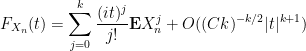
Consider the sum 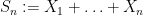


then 


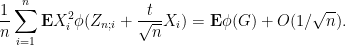
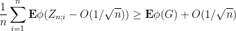
In the previous set of notes, we were able to establish various tail bounds on

and if the original distribution 

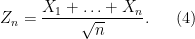
for some absolute constants 
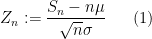
Now we look at the distribution of
Theorem 1 (Central limit theorem) Let
,
.
Exercise 2 Show that
of
, the quantities
and
are almost independent of each other, since the bulk of the sum
is determined by those
with
. Now make this intuition precise.)
Exercise 3 Use Stirling’s formula from Notes 0a to verify the central limit theorem in the case when
and
Exercise 4 Use Exercise 9 from Notes 1 to verify the central limit theorem in the case when
Note we are only discussing the case of real iid random variables. The case of complex random variables (or more generally, vector-valued random variables) is a little bit more complicated, and will be discussed later in this post.
The central limit theorem (and its variants, which we discuss below) are extremely useful tools in random matrix theory, in particular through the control they give on random walks (which arise naturally from linear functionals of random matrices). But the central limit theorem can also be viewed as a “commutative” analogue of various spectral results in random matrix theory (in particular, we shall see in later lectures that the Wigner semicircle law can be viewed in some sense as a “noncommutative” or “free” version of the central limit theorem). Because of this, the techniques used to prove the central limit theorem can often be adapted to be useful in random matrix theory. Because of this, we shall use these notes to dwell on several different proofs of the central limit theorem, as this provides a convenient way to showcase some of the basic methods that we will encounter again (in a more sophisticated form) when dealing with random matrices.
— 1. Reductions —
We first record some simple reductions one can make regarding the proof of the central limit theorem. Firstly, we observe scale invariance: if the central limit theorem holds for one random variable 


The other reduction we can make is truncation: to prove the central limit theorem for arbitrary random variables
Exercise 5 (Linearity of convergence) Let
be a finite-dimensional real or complex vector space,
be sequences of
be another pair of
be scalars converging to
respectively.
- If
converges in distribution to
, and at least one of
converges in distribution to
.
- If
.
- If
.
Show that the first part of the exercise can fail if
Now suppose that we have established the central limit theorem for bounded random variables, and want to extend to the unbounded case. Let 

Let 


converges in distribution to 

For such a sequence, we see from dominated convergence that 


converges in distribution to
Meanwhile, from dominated convergence again, 
converges in distribution to 
Remark 6 The truncation reduction is not needed for some proofs of the central limit theorem (notably the Fourier-analytic proof), but is very convenient for some of the other proofs that we will give here, and will also be used at several places in later notes.
By applying the scaling reduction after the truncation reduction, we observe that to prove the central limit theorem, it suffices to do so for random variables
— 2. The Fourier method —
Let us now give the standard Fourier-analytic proof of the central limit theorem. Given any real random variable 
Equivalently, 

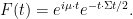
Example 7 The signed Bernoulli distribution has characteristic function
.
Exercise 8 Show that the normal distribution
has characteristic function
.
More generally, for a random variable 

where 


(or equivalently, by identifying 
More generally, one can define the characteristic function on any finite dimensional real or complex vector space 
The characteristic function is clearly bounded in magnitude by 
Exercise 9 (Riemann-Lebesgue lemma) Show that if
as
. Show that the claim can fail when the absolute continuity hypothesis is dropped.
Exercise 10 Show that the characteristic function
Let 
which thus interprets the characteristic function of a real random variable
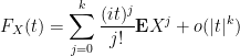
Exercise 11 (Taylor expansion of characteristic function) Let
moment for some
. Show that
times continuously differentiable, and one has the partial Taylor expansion
where
is a quantity that goes to zero as
, times
. In particular, we have
for all
.

Exercise 12 Establish (7) in the case that
Note that the characteristic function depends only on the distribution of 


Theorem 13 (Lévy continuity theorem, special case) Let
- (i)
converges pointwise to
- (ii)
Proof: Without loss of generality we may take 
The implication of (i) from (ii) is immediate from (6) and the definition of convergence in distribution (see Definition 10 of Notes 0), since the function 
Now suppose that (i) holds, and we wish to show that (ii) holds. By Exercise 23(iv) of Notes 0, it suffices to show that

whenever 

where

is a Schwartz function, and is in particular absolutely integrable (see e.g. these lecture notes of mine). From the Fubini-Tonelli theorem, we thus have

and similarly for

Remark 14 Setting
for all
Exercise 15 (Lévy’s continuity theorem, full version) Let
. Show that the following are equivalent:
- (i)
- (ii)
- (iii)
- (iv)
Hint: To get from (ii) to the other conclusions, use Prokhorov’s theorem and Theorem 13. To get back to (ii) from (i), use (8) for a suitable Schwartz function
Remark 16 Lévy’s continuity theorem is very similar in spirit to Weyl’s criterion in equidistribution theory.
Exercise 17 (Esséen concentration inequality) Let
,
, show that
for some constant
depending only on
and
. (Hint: Use (8) for a suitable Schwartz function
.

In Fourier analysis, we learn that the Fourier transform is a particularly well-suited tool for studying convolutions. The probability theory analogue of this fact is that characteristic functions are a particularly well-suited tool for studying sums of independent random variables. More precisely, we have
Exercise 18 (Fourier identities) Let
for all
. Also, for any scalar
, one has
and more generally, for any linear transformation
, one has


Remark 19 Note that this identity (10), combined with Exercise 8 and Remark 14, gives a quick alternate proof of Exercise 9 from Notes 1.
In particular, in the normalised setting (4), we have the simple relationship

that describes the characteristic function of
We now have enough machinery to give a quick proof of the central limit theorem:
Proof: (Proof of Theorem 1) We may normalise
for sufficiently small

for sufficiently small
as 
Exercise 20 (Vector-valued central limit theorem) Let
be a random variable taking values in
to be the
matrix
whose
entry is the covariance
.
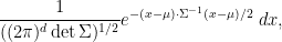
- Show that the covariance matrix is positive semi-definite real symmetric.
- Conversely, given any positive definite real symmetric
, show that the normal distribution
, given by the absolutely continuous measure
has mean
, and has a characteristic function given by
How would one define the normal distribution
- If
is the sum of
, show that
converges in distribution to
.
Exercise 21 (Complex central limit theorem) Let
, whose real and imaginary parts have variance
and covariance
.
Exercise 22 (Lindeberg central limit theorem) Let
be a sequence of independent (but not necessarily identically distributed) real random variables, normalised to have mean zero and variance one. Assume the (strong) Lindeberg condition
where
is the truncation of
to large values. Show that as
converges in distribution to

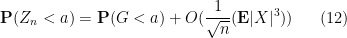
A more sophisticated version of the Fourier-analytic method gives a more quantitative form of the central limit theorem, namely the Berry-Esséen theorem.
Theorem 23 (Berry-Esséen theorem) Let
, where
are iid copies of
uniformly for all
, where
, and the implied constant is absolute.
Proof: (Optional) Write 

for all 

Let 

![{[-c,c]}](https://s0.wp.com/latex.php?latex=%7B%5B-c%2Cc%5D%7D&bg=ffffff&fg=000000&s=0&c=20201002)

![{1_{(-\infty,0]}}](https://s0.wp.com/latex.php?latex=%7B1_%7B%28-%5Cinfty%2C0%5D%7D%7D&bg=ffffff&fg=000000&s=0&c=20201002)
![\displaystyle \varphi(x) := \int_{\bf R} 1_{(-\infty,0]}(x - \varepsilon y) \eta(y)\ dy.](https://s0.wp.com/latex.php?latex=%5Cdisplaystyle+%5Cvarphi%28x%29+%3A%3D+%5Cint_%7B%5Cbf+R%7D+1_%7B%28-%5Cinfty%2C0%5D%7D%28x+-+%5Cvarepsilon+y%29+%5Ceta%28y%29%5C+dy.&bg=ffffff&fg=000000&s=0&c=20201002)
Observe that
We claim that it suffices to show that

for every 

thus our task is to show that 
Let 


and thus by (13)


Meanwhile, from (14) and an integration by parts we see that

From the bounded density of 

Putting all this together, we see that

A similar argument gives a lower bound

and so

Taking suprema over

If 


It remains to establish (13). Applying (8), it suffices to show that

Now we estimate each of the various expressions. Standard Fourier-analytic computations show that
![\displaystyle \hat \varphi(t) = \hat 1_{(-\infty,a]}(t) \hat \eta(\varepsilon t)](https://s0.wp.com/latex.php?latex=%5Cdisplaystyle+%5Chat+%5Cvarphi%28t%29+%3D+%5Chat+1_%7B%28-%5Cinfty%2Ca%5D%7D%28t%29+%5Chat+%5Ceta%28%5Cvarepsilon+t%29&bg=ffffff&fg=000000&s=0&c=20201002)
and that
![\displaystyle \hat 1_{(-\infty,a]}(t) = O( \frac{1}{1+|t|} ).](https://s0.wp.com/latex.php?latex=%5Cdisplaystyle+%5Chat+1_%7B%28-%5Cinfty%2Ca%5D%7D%28t%29+%3D+O%28+%5Cfrac%7B1%7D%7B1%2B%7Ct%7C%7D+%29.&bg=ffffff&fg=000000&s=0&c=20201002)
Since 

From Taylor expansion we have
for any

and in particular

if 

if 

(say) if
Exercise 24 Show that the error terms here are sharp (up to constants) when
— 3. The moment method —
The above Fourier-analytic proof of the central limit theorem is one of the quickest (and slickest) proofs available for this theorem, and is accordingly the “standard” proof given in probability textbooks. However, it relies quite heavily on the Fourier-analytic identities in Exercise 18, which in turn are extremely dependent on both the commutative nature of the situation (as it uses the identity 

The most elementary (but still remarkably effective) method available in this regard is the moment method, which we have already used in the previous notes, which seeks to understand the distribution of a random variable 
We first need an analogue of the Lévy continuity theorem. Here we encounter a technical issue: whereas the Fourier phases 

Theorem 25 (Moment continuity theorem) Let
- (i) For every
,
converges pointwise to
.
- (ii)
Proof: We first show how (ii) implies (i). Let 
![{[-1,1]}](https://s0.wp.com/latex.php?latex=%7B%5B-1%2C1%5D%7D&bg=ffffff&fg=000000&s=0&c=20201002)
![{[-2,2]}](https://s0.wp.com/latex.php?latex=%7B%5B-2%2C2%5D%7D&bg=ffffff&fg=000000&s=0&c=20201002)


Conversely, suppose (i) is true. From the uniform subgaussian hypothesis, the 


uniformly in

Then letting 


Remark 26 One corollary of Theorem 25 is that the distribution of a subgaussian random variable is uniquely determined by its moments (actually, this could already be deduced from Exercise 12 and Remark 14). The situation can fail for distributions with slower tails, for much the same reason that a smooth function is not determined by its derivatives at one point if that function is not analytic.
The Fourier inversion formula provides an easy way to recover the distribution from the characteristic function. Recovering a distribution from its moments is more difficult, and sometimes requires tools such as analytic continuation; this problem is known as the inverse moment problem and will not be discussed here.
To prove the central limit theorem, we know from the truncation method that we may assume without loss of generality that

for all
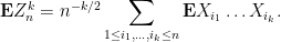
The moments 
Exercise 27 Let
when
So now we need to compute 
To understand this expression, let us first look at some small values of
- For
, this expression is trivially
- For
, this expression is trivially
- For
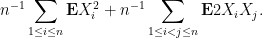
, we can split this expression into the diagonal and off-diagonal components:
Each summand in the first sum is
have mean zero and are independent. So the second moment
is
- For
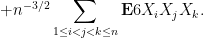
, we have a similar expansion
The summands in the latter two sums vanish because of the (joint) independence and mean zero hypotheses. The summands in the first sum need not vanish, but are
, which is asymptotically negligible, so the third moment
goes to
- For
, the expansion becomes quite complicated:
Again, most terms vanish, except for the first sum, which is
and is asymptotically negligible, and the sum
, which by the independence and unit variance assumptions works out to
. Thus the fourth moment
goes to
(as it should).


Now we tackle the general case. Ordering the indices 


where 

The total number of such terms depends only on 
As we already saw from the small 


On the other hand, the total number of summands in (17) is clearly at most 


and the main term is happily equal to the moment
— 4. The Lindeberg swapping trick —
The moment method proof of the central limit theorem that we just gave consisted of four steps:
- (Truncation and normalisation step) A reduction to the case when
- (Inverse moment step) A reduction to a computation of asymptotic moments
.
- (Analysis step) Showing that most terms in the expansion of this asymptotic moment were zero, or went to zero as
- (Algebra step) Using enumerative combinatorics to compute the remaining terms in the expansion.
In this particular case, the enumerative combinatorics was very classical and easy – it was basically asking for the number of ways one can place 

However, when we apply the moment method to more advanced problems, the enumerative combinatorics can become more non-trivial, requiring a fair amount of combinatorial and algebraic computation. The algebraic miracle that occurs at the end of the argument can then seem like a very fortunate but inexplicable coincidence, making the argument somehow unsatisfying despite being rigorous.
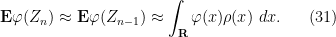
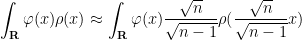
In a 1922 paper, Lindeberg observed that there was a very simple way to decouple the algebraic miracle from the analytic computations, so that all relevant algebraic identities only need to be verified in the special case of gaussian random variables, in which everything is much easier to compute. This Lindeberg swapping trick (or Lindeberg replacement trick) will be very useful in the later theory of random matrices, so we pause to give it here in the simple context of the central limit theorem.
The basic idea is follows. We repeat the truncation-and-normalisation and inverse moment steps in the preceding argument. Thus, 

Now let 
already has the same distribution as 

Now we perform the analysis part of the moment method argument again. We can expand 


But by hypothesis, the second moments of 
This is almost exactly the same proof as in the previous section, but note that we did not need to compute the multinomial coefficient
To put it another way, the Lindeberg replacement trick factors a universal limit theorem, such as the central limit theorem, into two components:
- A universality or invariance result, which shows that the distribution (or other statistics, such as moments) of some random variable
is asymptotically unchanged in the limit
- The gaussian case, which computes the asymptotic distribution (or other statistic) of
in the case when
The former type of result tends to be entirely analytic in nature (basically, one just needs to show that all error terms that show up when swapping
— 5. Individual swapping —
In the above argument, we swapped all the original input variables
Theorem 28 (Berry-Esséen theorem, weak form) Let
where

Proof: Let 

We telescope this (using linearity of expectation) as
where

is a partially swapped version of

uniformly for 
 and
and  , where
To exploit this, we use Taylor expansion with remainder to write

and


where the implied constants depend on 


and the claim follows. (Note from Hölder’s inequality that 
Remark 29 The above argument relied on Taylor expansion, and the hypothesis that the moments of
), and more smoothness on
factor on the right-hand side. Thus we see that we expect swapping methods to become more powerful when more moments are matching. We will see this when we discuss the four moment theorem of Van Vu and myself in later lectures, which (very) roughly speaking asserts that the spectral statistics of two random matrices are asymptotically indistinguishable if their coefficients have matching moments to fourth order.
Theorem 28 is easily implied by Theorem 23 and an integration by parts. In the reverse direction, let us see what Theorem 28 tells us about the cumulative distribution function

of

where ![{(-\infty,a]}](https://s0.wp.com/latex.php?latex=%7B%28-%5Cinfty%2Ca%5D%7D&bg=ffffff&fg=000000&s=0&c=20201002)
![{(-\infty,a+\varepsilon]}](https://s0.wp.com/latex.php?latex=%7B%28-%5Cinfty%2Ca%2B%5Cvarepsilon%5D%7D&bg=ffffff&fg=000000&s=0&c=20201002)

On the other hand, as

and so

A very similar argument gives the matching lower bound, thus
Optimising in

Comparing this with Theorem 23 we see that we have lost an exponent of 
On the other hand there is another method that can recover this loss while still avoiding Fourier-analytic techniques; we turn to this topic next.
— 6. Stein’s method —
Stein’s method, introduced by Charles Stein in 1970 (who should not be confused with a number of other eminent mathematicians with this surname, including my advisor), is a powerful method to show convergence in distribution to a special distribution, such as the gaussian. In several recent papers, this method has been used to control several expressions of interest in random matrix theory (e.g. the distribution of moments, or of the Stieltjes transform.) We will not use it much in this course, but this method is of independent interest, so I will briefly discuss (a very special case of) it here.
The probability density function 

One can take adjoints of this, and conclude (after an integration by parts) that 
for any continuously differentiable 


whenever 
It turns out that the converse is true: if

whenever
Theorem 30 (Stein continuity theorem) Let
- (i)
converges to zero whenever
is continuously differentiable with
- (ii)
Proof: To show that (ii) implies (i), it is not difficult to use the uniform bounded second moment hypothesis and a truncation argument to show that 
Now we establish the converse. It suffices to show that

whenever
Trivially, the function 
Comparing this with (22), one may thus hope to find a representation of the form

for some continuously differentiable
(One could dub

By completing the square, we see that 


which when inserted back into (24) gives the boundedness of
we see on differentiation under the integral sign (and using the Lipschitz nature of 


Applying (24) with 

By the hypothesis (i), the right-hand side goes to zero, hence the left-hand side does also, and the claim follows.
The above theorem gave only a qualitative result (convergence in distribution), but the proof is quite quantitative, and can be used to in particular to give Berry-Esséen type results. To illustrate this, we begin with a strengthening of Theorem 28 that reduces the number of derivatives of
Theorem 31 (Berry-Esséen theorem, less weak form) Let
where

Proof: Set 
Let

We expand 


where ![{[0,1]}](https://s0.wp.com/latex.php?latex=%7B%5B0%2C1%5D%7D&bg=ffffff&fg=000000&s=0&c=20201002)


Another application of independendence gives
so we may rewrite (28) as

Recall from the proof of Theorem 30 that 


and the claim follows from Hölder’s inequality.
This improvement already reduces the 
Theorem 32 (Berry-Esséen theorem, bounded case) Let
whenever
, where

Proof: Write ![{\phi := 1_{(-\infty,a]}}](https://s0.wp.com/latex.php?latex=%7B%5Cphi+%3A%3D+1_%7B%28-%5Cinfty%2Ca%5D%7D%7D&bg=ffffff&fg=000000&s=0&c=20201002)

Let 


and by arguing as in the proof of Theorem 31, we can write the right-hand side as
From (24),

The 
and so we conclude that
Since

applying the second inequality and using independence to once again eliminate the 
which implies (by another appeal to the non-increasing nature of

or in other words that

Similarly, using the lower bound inequalities, one has

Moving 
Actually, one can use Stein’s method to obtain the full Berry-Esséen theorem, but the computations get somewhat technical, requiring an induction on
— 7. Predecessor comparison —
Suppose one had never heard of the normal distribution, but one still suspected the existence of the central limit theorem – thus, one thought that the sequence
Certainly in the case of Bernoulli distributions, one could work explicitly using Stirling’s formula (see Exercise 3), and the Fourier-analytic method would also eventually work. Let us now give a third way to (heuristically) derive the normal distribution as the limit of the central limit theorem. The idea is to compare 

(normalising 


Now let us try to combine this with (30). We assume


Taking expectations, and using the independence of

Up to errors of 


Changing variables for the first term on the right hand side, and integrating by parts for the second term, we have
Since

Taylor expansion gives

which leads us to the heuristic ODE

where 

Observe that 

which is (21), and can be solved by standard ODE methods as 

The above argument was not rigorous, but one can make it so with a significant amount of PDE machinery. If we view 

which is a linear parabolic equation that is fortunate enough that it can be solved exactly (indeed, it is not difficult to transform this equation to the linear heat equation by some straightforward changes of variable). Using the spectral theory of the Ornstein-Uhlenbeck operator
This argument does, though highlight two ideas which we will see again in later notes when studying random matrices. Firstly, that it is profitable to study the distribution of some random object

87 comments
Comments feed for this article
9 December, 2022 at 3:57 am
Solved – Central limit theorem proof not using characteristic functions - Everything about Math, Questions, Topics
[…] Also, Stein's method is nothing short of black magic! You can find an exposition of the proof in section 6 of this link. You'll find other proofs of the CLT in the link as […]
1 August, 2023 at 3:23 pm
The Square Root Cancellation Heuristic | George Shakan
[…] This is the so-called square root cancellation. If we take a random vector of dimension with randomly generated entries, we expect the order of the sum to be . Here , and it is a general phenomenon that most of the sums will lie between, say, and . This general principle goes much deeper than vectors and turns out to be very well-studied concept in several areas of mathematics (see this post for Number Theory or this post for Probability). […]
17 April, 2024 at 6:31 am
Anonymous
Dear Terry,
There is maybe a typo immediately after (26) when writing the “completing the square”.
[Sorry, I don’t see any typo; could you be more specific? -T]