
You are currently browsing the category archive for the ‘math.CA’ category.
Let 

![{H[X]}](https://s0.wp.com/latex.php?latex=%7BH%5BX%5D%7D&bg=ffffff&fg=000000&s=0&c=20201002)
![\displaystyle H[X] = -\sum_{s \in S} {\bf P}[X = s] \log {\bf P}[X = s].](https://s0.wp.com/latex.php?latex=%5Cdisplaystyle+H%5BX%5D+%3D+-%5Csum_%7Bs+%5Cin+S%7D+%7B%5Cbf+P%7D%5BX+%3D+s%5D+%5Clog+%7B%5Cbf+P%7D%5BX+%3D+s%5D.&bg=ffffff&fg=000000&s=0&c=20201002)
Lemma 1 (Gibbs variational formula) Letbe a function. Then
![\displaystyle \log \sum_{s \in S} \exp(f(s)) = \sup_X {\bf E} f(X) + {\bf H}[X]. \ \ \ \ \ (1)](https://s0.wp.com/latex.php?latex=%5Cdisplaystyle++%5Clog+%5Csum_%7Bs+%5Cin+S%7D+%5Cexp%28f%28s%29%29+%3D+%5Csup_X+%7B%5Cbf+E%7D+f%28X%29+%2B+%7B%5Cbf+H%7D%5BX%5D.+%5C+%5C+%5C+%5C+%5C+%281%29&bg=ffffff&fg=000000&s=0&c=20201002)
Proof: Note that shifting 


![\displaystyle 0 = \sup_X \sum_{s \in S} {\bf P}[X = s] \log {\bf P}[Y = s] -\sum_{s \in S} {\bf P}[X = s] \log {\bf P}[X = s].](https://s0.wp.com/latex.php?latex=%5Cdisplaystyle++0+%3D+%5Csup_X+%5Csum_%7Bs+%5Cin+S%7D+%7B%5Cbf+P%7D%5BX+%3D+s%5D+%5Clog+%7B%5Cbf+P%7D%5BY+%3D+s%5D+-%5Csum_%7Bs+%5Cin+S%7D+%7B%5Cbf+P%7D%5BX+%3D+s%5D+%5Clog+%7B%5Cbf+P%7D%5BX+%3D+s%5D.&bg=ffffff&fg=000000&s=0&c=20201002)
 , where
  denotes Kullback-Leibler divergence. One can also interpret this inequality as a special case of the Fenchel–Young inequality relating the conjugate convex functions
  and
and  .)
.) 
In this note I would like to use this variational formula (which is also known as the Donsker-Varadhan variational formula) to give another proof of the following inequality of Carbery.
Theorem 2 (Generalized Cauchy-Schwarz inequality) Let, let
be finite non-empty sets, and let
be functions for each
. Let
and
be positive functions for each
where
is the quantity
where
is the set of all tuples
such that
for

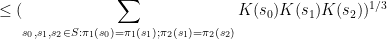
Thus for instance, the identity is trivial for 

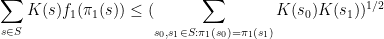

 the inequality reads

 , the existing proofs require the “tensor power trick” in order to reduce to the case when the
  are step functions (in which case the inequality can be proven elementarily, as discussed in the above paper of Carbery).
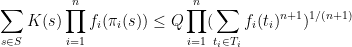
We now prove this inequality. We write 


![\displaystyle \sup_X {\bf E} k(X) + \sum_{i=1}^n g_i(\pi_i(X)) + {\bf H}[X]](https://s0.wp.com/latex.php?latex=%5Cdisplaystyle++%5Csup_X+%7B%5Cbf+E%7D+k%28X%29+%2B+%5Csum_%7Bi%3D1%7D%5En+g_i%28%5Cpi_i%28X%29%29+%2B+%7B%5Cbf+H%7D%5BX%5D+&bg=ffffff&fg=000000&s=0&c=20201002)
![\displaystyle \leq \frac{1}{n+1} \sup_{(X_0,\dots,X_n)} {\bf E} k(X_0)+\dots+k(X_n) + {\bf H}[X_0,\dots,X_n]](https://s0.wp.com/latex.php?latex=%5Cdisplaystyle++%5Cleq+%5Cfrac%7B1%7D%7Bn%2B1%7D+%5Csup_%7B%28X_0%2C%5Cdots%2CX_n%29%7D+%7B%5Cbf+E%7D+k%28X_0%29%2B%5Cdots%2Bk%28X_n%29+%2B+%7B%5Cbf+H%7D%5BX_0%2C%5Cdots%2CX_n%5D+&bg=ffffff&fg=000000&s=0&c=20201002)
![\displaystyle + \frac{1}{n+1} \sum_{i=1}^n \sup_{Y_i} (n+1) {\bf E} g_i(Y_i) + {\bf H}[Y_i]](https://s0.wp.com/latex.php?latex=%5Cdisplaystyle++%2B+%5Cfrac%7B1%7D%7Bn%2B1%7D+%5Csum_%7Bi%3D1%7D%5En+%5Csup_%7BY_i%7D+%28n%2B1%29+%7B%5Cbf+E%7D+g_i%28Y_i%29+%2B+%7B%5Cbf+H%7D%5BY_i%5D&bg=ffffff&fg=000000&s=0&c=20201002) ranges over random variables taking values in ,
ranges over random variables taking values in ,  range over tuples of random variables taking values in , and
  range over random variables taking values in
  . Comparing the suprema, the claim now reduces to
Lemma 3 (Conditional expectation computation) Let, where each
has the same distribution as
![\displaystyle {\bf H}[X_0,\dots,X_n] = (n+1) {\bf H}[X]](https://s0.wp.com/latex.php?latex=%5Cdisplaystyle++%7B%5Cbf+H%7D%5BX_0%2C%5Cdots%2CX_n%5D+%3D+%28n%2B1%29+%7B%5Cbf+H%7D%5BX%5D+&bg=ffffff&fg=000000&s=0&c=20201002)
![\displaystyle - {\bf H}[\pi_1(X)] - \dots - {\bf H}[\pi_n(X)].](https://s0.wp.com/latex.php?latex=%5Cdisplaystyle+-+%7B%5Cbf+H%7D%5B%5Cpi_1%28X%29%5D+-+%5Cdots+-+%7B%5Cbf+H%7D%5B%5Cpi_n%28X%29%5D.&bg=ffffff&fg=000000&s=0&c=20201002)
Proof: We induct on 


![\displaystyle {\bf H}[X_0,\dots,X_{n-1}] = n {\bf H}[X] - {\bf H}[\pi_1(X)] - \dots - {\bf H}[\pi_{n-1}(X)].](https://s0.wp.com/latex.php?latex=%5Cdisplaystyle++%7B%5Cbf+H%7D%5BX_0%2C%5Cdots%2CX_%7Bn-1%7D%5D+%3D+n+%7B%5Cbf+H%7D%5BX%5D+-+%7B%5Cbf+H%7D%5B%5Cpi_1%28X%29%5D+-+%5Cdots+-+%7B%5Cbf+H%7D%5B%5Cpi_%7Bn-1%7D%28X%29%5D.&bg=ffffff&fg=000000&s=0&c=20201002)
 has the same distribution as
  . For each value
  attained by , we can take conditionally independent copies of
  and conditioned to the events
  and
and  respectively, and then concatenate them to form a tuple in , with
  a further copy of that is conditionally independent of relative to
  . One can the use the entropy chain rule to compute
 ![\displaystyle {\bf H}[X_0,\dots,X_n] = {\bf H}[\pi_n(X_n)] + {\bf H}[X_0,\dots,X_n| \pi_n(X_n)]](https://s0.wp.com/latex.php?latex=%5Cdisplaystyle++%7B%5Cbf+H%7D%5BX_0%2C%5Cdots%2CX_n%5D+%3D+%7B%5Cbf+H%7D%5B%5Cpi_n%28X_n%29%5D+%2B+%7B%5Cbf+H%7D%5BX_0%2C%5Cdots%2CX_n%7C+%5Cpi_n%28X_n%29%5D&bg=ffffff&fg=000000&s=0&c=20201002)
![\displaystyle = {\bf H}[\pi_n(X_n)] + {\bf H}[X_0,\dots,X_{n-1}| \pi_n(X_n)] + {\bf H}[X_n| \pi_n(X_n)]](https://s0.wp.com/latex.php?latex=%5Cdisplaystyle++%3D+%7B%5Cbf+H%7D%5B%5Cpi_n%28X_n%29%5D+%2B+%7B%5Cbf+H%7D%5BX_0%2C%5Cdots%2CX_%7Bn-1%7D%7C+%5Cpi_n%28X_n%29%5D+%2B+%7B%5Cbf+H%7D%5BX_n%7C+%5Cpi_n%28X_n%29%5D+&bg=ffffff&fg=000000&s=0&c=20201002)
![\displaystyle = {\bf H}[\pi_n(X)] + {\bf H}[X_0,\dots,X_{n-1}| \pi_n(X_{n-1})] + {\bf H}[X_n| \pi_n(X_n)]](https://s0.wp.com/latex.php?latex=%5Cdisplaystyle++%3D+%7B%5Cbf+H%7D%5B%5Cpi_n%28X%29%5D+%2B+%7B%5Cbf+H%7D%5BX_0%2C%5Cdots%2CX_%7Bn-1%7D%7C+%5Cpi_n%28X_%7Bn-1%7D%29%5D+%2B+%7B%5Cbf+H%7D%5BX_n%7C+%5Cpi_n%28X_n%29%5D+&bg=ffffff&fg=000000&s=0&c=20201002)
![\displaystyle = {\bf H}[\pi_n(X)] + ({\bf H}[X_0,\dots,X_{n-1}] - {\bf H}[\pi_n(X_{n-1})])](https://s0.wp.com/latex.php?latex=%5Cdisplaystyle++%3D+%7B%5Cbf+H%7D%5B%5Cpi_n%28X%29%5D+%2B+%28%7B%5Cbf+H%7D%5BX_0%2C%5Cdots%2CX_%7Bn-1%7D%5D+-+%7B%5Cbf+H%7D%5B%5Cpi_n%28X_%7Bn-1%7D%29%5D%29+&bg=ffffff&fg=000000&s=0&c=20201002)
![\displaystyle + ({\bf H}[X_n] - {\bf H}[\pi_n(X_n)])](https://s0.wp.com/latex.php?latex=%5Cdisplaystyle+%2B+%28%7B%5Cbf+H%7D%5BX_n%5D+-+%7B%5Cbf+H%7D%5B%5Cpi_n%28X_n%29%5D%29+&bg=ffffff&fg=000000&s=0&c=20201002)
![\displaystyle ={\bf H}[X_0,\dots,X_{n-1}] + {\bf H}[X_n] - {\bf H}[\pi_n(X_n)]](https://s0.wp.com/latex.php?latex=%5Cdisplaystyle++%3D%7B%5Cbf+H%7D%5BX_0%2C%5Cdots%2CX_%7Bn-1%7D%5D+%2B+%7B%5Cbf+H%7D%5BX_n%5D+-+%7B%5Cbf+H%7D%5B%5Cpi_n%28X_n%29%5D&bg=ffffff&fg=000000&s=0&c=20201002)
With a little more effort, one can replace
In my previous post, I walked through the task of formally deducing one lemma from another in Lean 4. The deduction was deliberately chosen to be short and only showcased a small number of Lean tactics. Here I would like to walk through the process I used for a slightly longer proof I worked out recently, after seeing the following challenge from Damek Davis: to formalize (in a civilized fashion) the proof of the following lemma:
Lemma. Let
and
be sequences of real numbers indexed by natural numbers
, with
non-increasing and
non-negative. Suppose also that
for all
. Then
for all
.
Here I tried to draw upon the lessons I had learned from the PFR formalization project, and to first set up a human readable proof of the lemma before starting the Lean formalization – a lower-case “blueprint” rather than the fancier Blueprint used in the PFR project. The main idea of the proof here is to use the telescoping series identity
Since 

but by the monotone hypothesis on 

This is already a human-readable proof, but in order to formalize it more easily in Lean, I decided to rewrite it as a chain of inequalities, starting at 

(by field identities)

(by the formula for summing a constant)

(by the monotone hypothesis)

(by the hypothesis
(by telescoping series)

(by the non-negativity of
I decided that this was a good enough blueprint for me to work with. The next step is to formalize the statement of the lemma in Lean. For this quick project, it was convenient to use the online Lean playground, rather than my local IDE, so the screenshots will look a little different from those in the previous post. (If you like, you can follow this tour in that playground, by clicking on the screenshots of the Lean code.) I start by importing Lean’s math library, and starting an example of a statement to state and prove:

Now we have to declare the hypotheses and variables. The main variables here are the sequences a, D from the natural numbers ℕ to the reals ℝ. (One can choose to “hardwire” the non-negativity hypothesis into the D take values in the nonnegative reals 
NNReal in Lean), but this turns out to be inconvenient, because the laws of algebra and summation that we will need are clunkier on the non-negative reals (which are not even a group) than on the reals (which are a field). So we add in the variables:

Now we add in the hypotheses, which in Lean convention are usually given names starting with h. This is fairly straightforward; the one thing is that the property of being monotone decreasing already has a name in Lean’s Mathlib, namely Antitone, and it is generally a good idea to use the Mathlib provided terminology (because that library contains a lot of useful lemmas about such terms).

One thing to note here is that Lean is quite good at filling in implied ranges of variables. Because a and D have the natural numbers ℕ as their domain, the dummy variable k in these hypotheses is automatically being quantified over ℕ. We could have made this quantification explicit if we so chose, for instance using ∀ k : ℕ, 0 ≤ D k instead of ∀ k, 0 ≤ D k, but it is not necessary to do so. Also note that Lean does not require parentheses when applying functions: we write D k here rather than D(k) (which in fact does not compile in Lean unless one puts a space between the D and the parentheses). This is slightly different from standard mathematical notation, but is not too difficult to get used to.
This looks like the end of the hypotheses, so we could now add a colon to move to the conclusion, and then add that conclusion:

This is a perfectly fine Lean statement. But it turns out that when proving a universally quantified statement such as ∀ k, a k ≤ D 0 / (k + 1), the first step is almost always to open up the quantifier to introduce the variable k (using the Lean command intro k). Because of this, it is slightly more efficient to hide the universal quantifier by placing the variable k in the hypotheses, rather than in the quantifier (in which case we have to now specify that it is a natural number, as Lean can no longer deduce this from context):

At this point Lean is complaining of an unexpected end of input: the example has been stated, but not proved. We will temporarily mollify Lean by adding a sorry as the purported proof:

Now Lean is content, other than giving a warning (as indicated by the yellow squiggle under the example) that the proof contains a sorry.
It is now time to follow the blueprint. The Lean tactic for proving an inequality via chains of other inequalities is known as calc. We use the blueprint to fill in the calc that we want, leaving the justifications of each step as “sorry”s for now:

Here, we “open“ed the Finset namespace in order to easily access Finset‘s range function, with range k basically being the finite set of natural numbers 
open“ed the BigOperators namespace to access the familiar ∑ notation for (finite) summation, in order to make the steps in the Lean code resemble the blueprint as much as possible. One could avoid opening these namespaces, but then expressions such as ∑ i in range (k+1), a i would instead have to be written as something like Finset.sum (Finset.range (k+1)) (fun i ↦ a i), which looks a lot less like like standard mathematical writing. The proof structure here may remind some readers of the “two column proofs” that are somewhat popular in American high school geometry classes.
Now we have six sorries to fill. Navigating to the first sorry, Lean tells us the ambient hypotheses, and the goal that we need to prove to fill that sorry:

The ⊢ symbol here is Lean’s marker for the goal. The uparrows ↑ are coercion symbols, indicating that the natural number k has to be converted to a real number in order to interact via arithmetic operations with other real numbers such as a k, but we can ignore these coercions for this tour (for this proof, it turns out Lean will basically manage them automatically without need for any explicit intervention by a human).
The goal here is a self-evident algebraic identity; it involves division, so one has to check that the denominator is non-zero, but this is self-evident. In Lean, a convenient way to establish algebraic identities is to use the tactic field_simp to clear denominators, and then ring to verify any identity that is valid for commutative rings. This works, and clears the first sorry:

field_simp, by the way, is smart enough to deduce on its own that the denominator k+1 here is manifestly non-zero (and in fact positive); no human intervention is required to point this out. Similarly for other “clearing denominator” steps that we will encounter in the other parts of the proof.
Now we navigate to the next `sorry`. Lean tells us the hypotheses and goals:

We can reduce the goal by canceling out the common denominator ↑k+1. Here we can use the handy Lean tactic congr, which tries to match two sides of an equality goal as much as possible, and leave any remaining discrepancies between the two sides as further goals to be proven. Applying congr, the goal reduces to

Here one might imagine that this is something that one can prove by induction. But this particular sort of identity – summing a constant over a finite set – is already covered by Mathlib. Indeed, searching for Finset, sum, and const soon leads us to the Finset.sum_const lemma here. But there is an even more convenient path to take here, which is to apply the powerful tactic simp, which tries to simplify the goal as much as possible using all the “simp lemmas” Mathlib has to offer (of which Finset.sum_const is an example, but there are thousands of others). As it turns out, simp completely kills off this identity, without any further human intervention:

Now we move on to the next sorry, and look at our goal:

congr doesn’t work here because we have an inequality instead of an equality, but there is a powerful relative gcongr of congr that is perfectly suited for inequalities. It can also open up sums, products, and integrals, reducing global inequalities between such quantities into pointwise inequalities. If we invoke gcongr with i hi (where we tell gcongr to use i for the variable opened up, and hi for the constraint this variable will satisfy), we arrive at a greatly simplified goal (and a new ambient variable and hypothesis):

Now we need to use the monotonicity hypothesis on a, which we have named ha here. Looking at the documentation for Antitone, one finds a lemma that looks applicable here:

One can apply this lemma in this case by writing apply Antitone.imp ha, but because ha is already of type Antitone, we can abbreviate this to apply ha.imp. (Actually, as indicated in the documentation, due to the way Antitone is defined, we can even just use apply ha here.) This reduces the goal nicely:

The goal is now very close to the hypothesis hi. One could now look up the documentation for Finset.range to see how to unpack hi, but as before simp can do this for us. Invoking simp at hi, we obtain

Now the goal and hypothesis are very close indeed. Here we can just close the goal using the linarith tactic used in the previous tour:

The next sorry can be resolved by similar methods, using the hypothesis hD applied at the variable i:

Now for the penultimate sorry. As in a previous step, we can use congr to remove the denominator, leaving us in this state:

This is a telescoping series identity. One could try to prove it by induction, or one could try to see if this identity is already in Mathlib. Searching for Finset, sum, and sub will locate the right tool (as the fifth hit), but a simpler way to proceed here is to use the exact? tactic we saw in the previous tour:

A brief check of the documentation for sum_range_sub' confirms that this is what we want. Actually we can just use apply sum_range_sub' here, as the apply tactic is smart enough to fill in the missing arguments:

One last sorry to go. As before, we use gcongr to cancel denominators, leaving us with

This looks easy, because the hypothesis hpos will tell us that D (k+1) is nonnegative; specifically, the instance hpos (k+1) of that hypothesis will state exactly this. The linarith tactic will then resolve this goal once it is told about this particular instance:

We now have a complete proof – no more yellow squiggly line in the example. There are two warnings though – there are two variables i and hi introduced in the proof that Lean’s “linter” has noticed are not actually used in the proof. So we can rename them with underscores to tell Lean that we are okay with them not being used:

This is a perfectly fine proof, but upon noticing that many of the steps are similar to each other, one can do a bit of “code golf” as in the previous tour to compactify the proof a bit:

With enough familiarity with the Lean language, this proof actually tracks quite closely with (an optimized version of) the human blueprint.
This concludes the tour of a lengthier Lean proving exercise. I am finding the pre-planning step of the proof (using an informal “blueprint” to break the proof down into extremely granular pieces) to make the formalization process significantly easier than in the past (when I often adopted a sequential process of writing one line of code at a time without first sketching out a skeleton of the argument). (The proof here took only about 15 minutes to create initially, although for this blog post I had to recreate it with screenshots and supporting links, which took significantly more time.) I believe that a realistic near-term goal for AI is to be able to fill in automatically a significant fraction of the sorts of atomic “sorry“s of the size one saw in this proof, allowing one to convert a blueprint to a formal Lean proof even more rapidly.
One final remark: in this tour I filled in the “sorry“s in the order in which they appeared, but there is actually no requirement that one does this, and once one has used a blueprint to atomize a proof into self-contained smaller pieces, one can fill them in in any order. Importantly for a group project, these micro-tasks can be parallelized, with different contributors claiming whichever “sorry” they feel they are qualified to solve, and working independently of each other. (And, because Lean can automatically verify if their proof is correct, there is no need to have a pre-existing bond of trust with these contributors in order to accept their contributions.) Furthermore, because the specification of a “sorry” someone can make a meaningful contribution to the proof by working on an extremely localized component of it without needing the mathematical expertise to understand the global argument. This is not particularly important in this simple case, where the entire lemma is not too hard to understand to a trained mathematician, but can become quite relevant for complex formalization projects.
I have just uploaded to the arXiv my paper “A Maclaurin type inequality“. This paper concerns a variant of the Maclaurin inequality for the elementary symmetric means
 real numbers
  . This inequality asserts that
 and are non-negative. It can be proven as a consequence of the Newton inequality
 and arbitrary real (in particular, here the
  are allowed to be negative). Note that the
  case of this inequality is just the arithmetic mean-geometric mean inequality
 to obtain another real-rooted polynomial, thanks to Rolle’s theorem; the key point is that this operation preserves all the elementary symmetric means up to
  ). One can think of Maclaurin’s inequality as providing a refined version of the arithmetic mean-geometric mean inequality on variables (which corresponds to the case
  ,
,  ).
).
Whereas Newton’s inequality works for arbitrary real 


On the other hand, it was observed by Gopalan and Yehudayoff that if two consecutive values 


However, if one inspects the bound (2) against the bounds (1) given by the key example, we see a mismatch – the right-hand side of (2) is larger than the left-hand side by a factor of about 

Unlike the previous arguments, we do not rely primarily on the arithmetic mean-geometric mean inequality. Instead, our primary tool is a new inequality 


We sketch the proof of the inequality (4) as follows. One can use some standard manipulations reduce to the case where 


 equal to and the other half equal to , thanks to the binomial theorem.
To prove this identity, we consider the polynomial
 , taking absolute values, using the triangle inequality, and then taking logarithms, we conclude that
 gives
gives 
A common task in analysis is to obtain bounds on sums


 is some simple region (such as an interval) in one or more dimensions, and is an explicit (and elementary) non-negative expression involving one or more variables (such as or
  , and possibly also some additional parameters. Often, one would be content with an order of magnitude upper bound such as

 (or
(or  or
or  ) to denote the bound
  for some constant
  ; sometimes one wishes to also obtain the matching lower bound, thus obtaining
 is synonymous with
  . Finally, one may wish to obtain a more precise bound, such as
 is a quantity that goes to zero as the parameters of the problem go to infinity (or some other limit). (For a deeper dive into asymptotic notation in general, see this previous blog post.)
Here are some typical examples of such estimation problems, drawn from recent questions on MathOverflow:
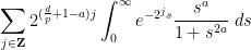
- (i) (From this question) If
and
, is the expression
finite? - (ii) (From this question) If
, how can one show that
- (iii) (From this question) Can one show that
asfor an explicit constant
, and what is this constant?

Compared to other estimation tasks, such as that of controlling oscillatory integrals, exponential sums, singular integrals, or expressions involving one or more unknown functions (that are only known to lie in some function spaces, such as an 
Somewhat in the spirit of this previous post on analysis problem solving strategies, I am going to try here to collect some general principles and techniques that I have found useful for these sorts of problems. As with the previous post, I hope this will be something of a living document, and encourage others to add their own tips or suggestions in the comments.
Jon Bennett and I have just uploaded to the arXiv our paper “Adjoint Brascamp-Lieb inequalities“. In this paper, we observe that the family of multilinear inequalities known as the Brascamp-Lieb inequalities (or Holder-Brascamp-Lieb inequalities) admit an adjoint formulation, and explore the theory of these adjoint inequalities and some of their consequences.
To motivate matters let us review the classical theory of adjoints for linear operators. If one has a bounded linear operator 


 (and similarly for
  ), one can show that
  has the same operator norm as
  .
.
There is a slightly different way to proceed using Hölder’s inequality. For sake of exposition let us make the simplifying assumption that 


 we obtain
  , and a similar argument also recovers the reverse inequality.
The first argument also extends to some extent to multilinear operators. For instance if one has a bounded bilinear operator 


 . It is also possible, formally at least, to adapt the Hölder inequality argument to reach the same conclusion.
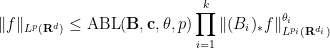
In this paper we observe that the Hölder inequality argument can be modified in the case of Brascamp-Lieb inequalities to obtain a different type of adjoint inequality. (Continuous) Brascamp-Lieb inequalities take the form

 and surjective linear maps
  , where
  are arbitrary non-negative measurable functions and
  is the best constant for which this inequality holds for all such . [There is also another inequality involving variances with respect to log-concave distributions that is also due to Brascamp and Lieb, but it is not related to the inequalities discussed here.] Well known examples of such inequalities include Hölder’s inequality and the sharp Young convolution inequality; another is the Loomis-Whitney inequality, the first non-trivial example of which is

 . There are also discrete analogues of these inequalities, in which the Euclidean spaces
  are replaced by discrete abelian groups, and the surjective linear maps
  are replaced by discrete homomorphisms.
The operation 


 and various exponents
  , where
  is the optimal constant for which the above inequality holds for all such ; informally, such inequalities control the norm of a non-negative function in terms of its marginals. It turns out that every Brascamp-Lieb inequality generates a family of adjoint Brascamp-Lieb inequalities (with the exponent
  being less than or equal to
  ). For instance, the adjoints of the Loomis-Whitney inequality (2) are the inequalities
 , all
, all  summing to , and all
  , where the
  exponents are defined by the formula
 are the marginals of :
One can derive these adjoint Brascamp-Lieb inequalities from their forward counterparts by a version of the Hölder inequality argument mentioned previously, in conjunction with the observation that the pushforward maps 
We have located a modest number of applications of the adjoint Brascamp-Lieb inequality (but hope that there will be more in the future):
- The inequalities become equalities at
; taking a derivative at this value (in the spirit of the replica trick in physics) we recover the entropic Brascamp-Lieb inequalities of Carlen and Cordero-Erausquin. For instance, the derivative of the adjoint Loomis-Whitney inequalities at
- The adjoint Loomis-Whitney inequalities, together with a few more applications of Hölder’s inequality, implies the log-concavity of the Gowers uniformity norms on non-negative functions, which was previously observed by Shkredov and by Manners.
- Averaging the adjoint Loomis-Whitney inequalities over coordinate systems gives reverse
norms or entropies of the
are chosen in a dimensionally consistent fashion).
We also record a number of variants of the adjoint Brascamp-Lieb inequalities, including discrete variants, and a reverse inequality involving 

The “epsilon-delta” nature of analysis can be daunting and unintuitive to students, as the heavy reliance on inequalities rather than equalities. But it occurred to me recently that one might be able to leverage the intuition one already has from “deals” – of the type one often sees advertised by corporations – to get at least some informal understanding of these concepts.
Take for instance the concept of an upper bound 


| Currency | We buy at | We sell at |
| |  |  |
 | – |  |
 |  | |
 | – |  |
Someone with an eye for spotting “deals” might now realize that one can actually buy 


Asymptotic estimates such as 

When it comes to the basic analysis concepts of convergence and continuity, one can similarly view these concepts as various economic transactions involving the buying and selling of accuracy. One could for instance imagine the following hypothetical range of products in which one would need to spend more money to obtain higher accuracy to measure weight in grams:
| Object | Accuracy | Price |
| Low-end kitchen scale |  gram gram |  |
| High-end bathroom scale |  grams grams |  |
| Low-end lab scale |  grams grams |  |
| High-end lab scale |  grams grams |  |
The concept of convergence 


| Status | Accuracy benefit | Eligibility |
| Basic status |  | |
| Bronze status |  |  |
| Silver status |  |  |
| Gold status |  |  |
 | | |
With this conceptual model, convergence means that any status level of accuracy can be unlocked if one’s number
In a similar vein, continuity becomes analogous to a conversion program, in which accuracy benefits from one company can be traded in for new accuracy benefits in another company. For instance, the continuity of the function 

| Accuracy benefit of to trade in | Accuracy benefit of  obtained obtained |
 |  |
 |  |
 |  |
| | |
Again, the point is that one can purchase any desired level of accuracy of
At present, the above conversion chart is only available at the single location 

In a similar vein, differentiability can be viewed as a deal in which one can trade in accuracy of the input for approximately linear behavior of the output; to oversimplify slightly, smoothness can similarly be viewed as a deal in which one trades in accuracy of the input for high-accuracy polynomial approximability of the output. Measurability of a set or function can be viewed as a deal in which one trades in a level of resolution for an accurate approximation of that set or function at the given resolution. And so forth.
Perhaps readers can propose some other examples of mathematical concepts being re-interpreted as some sort of economic transaction?
In orthodox first-order logic, variables and expressions are only allowed to take one value at a time; a variable 

However, the ability to allow expressions to become only partially specified is undeniably convenient, and also rather intuitive. A classic example here is that of the quadratic formula:


Strictly speaking, the expression 

or

or

in order to strictly adhere to this grammar. But none of these three reformulations are as compact or as conceptually clear as the original one. In a similar spirit, a mathematical English sentence such as


 which are used once and then discarded.
Another example of partially specified notation is the innocuous 


Below the fold I’ll try to assign a formal meaning to partially specified expressions such as (1), for instance allowing one to condense (2), (3), (4) to just
 or the little-o notation
  . We will explain how to do this at the end of this post.
A few months ago I posted a question about analytic functions that I received from a bright high school student, which turned out to be studied and resolved by de Bruijn. Based on this positive resolution, I thought I might try my luck again and list three further questions that this student asked which do not seem to be trivially resolvable.
- Does there exist a smooth function
which is nowhere analytic, but is such that the Taylor series
converges for every
? (Of course, this series would not then converge to
for each
- Is there a function
to infinite order in the following sense: for every polynomial
, there exists
for all
? Such a function would be rather pathological, perhaps resembling a space-filling curve. (Update: solved for smooth
- Is there a power series
that diverges everywhere (except at
), but which becomes pointwise convergent after dividing each of the monomials
into pieces
for some
summing absolutely to
, and then rearranging, i.e., there is some rearrangement
of
that is pointwise convergent for every
Feel free to post answers or other thoughts on these questions in the comments.
Louis Esser, Burt Totaro, Chengxi Wang, and myself have just uploaded to the arXiv our preprint “Varieties of general type with many vanishing plurigenera, and optimal sine and sawtooth inequalities“. This is an interdisciplinary paper that arose because in order to optimize a certain algebraic geometry construction it became necessary to solve a purely analytic question which, while simple, did not seem to have been previously studied in the literature. We were able to solve the analytic question exactly and thus fully optimize the algebraic geometry construction, though the analytic question may have some independent interest.
Let us first discuss the algebraic geometry application. Given a smooth complex 


 for some non-negative number
  , which is called the volume of the variety , which is an invariant that reveals some information about the birational geometry of . For instance, if the canonical line bundle is ample (or more generally, nef), this volume is equal to the intersection number
  (roughly speaking, the number of common zeroes of generic sections of the canonical line bundle); this is a special case of the asymptotic Riemann-Roch theorem. In particular, the volume is a natural number in this case. However, it is possible for the volume to also be fractional in nature. One can then ask: how small can the volume get without vanishing entirely? (By definition, varieties with non-vanishing volume are known as varieties of general type.)
It follows from a deep result obtained independently by Hacon–McKernan, Takayama and Tsuji that there is a uniform lower bound for the volume 


The space 


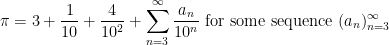
Now it is time to turn to the analytic side of the paper by describing the optimization problem that we solve. We consider the sawtooth function ![{g: {\bf R} \rightarrow (-1/2,1/2]}](https://s0.wp.com/latex.php?latex=%7Bg%3A+%7B%5Cbf+R%7D+%5Crightarrow+%28-1%2F2%2C1%2F2%5D%7D&bg=ffffff&fg=000000&s=0&c=20201002)

![{(-1/2,1/2]}](https://s0.wp.com/latex.php?latex=%7B%28-1%2F2%2C1%2F2%5D%7D&bg=ffffff&fg=000000&s=0&c=20201002)

 is bounded above by
  , we certainly have the trivial bound
 could attain the value of is if the probability measure was supported on half-integers, but in that case
  would vanish. For the algebraic geometry application discussed above one is then led to the following question: for a given choice of , what is the best upper bound
  on the quantity
  that holds for all probability measures ?
If one considers the deterministic case in which 

 . Thus we have
  is comparable to
  . In fact we were able to compute this quantity precisely:
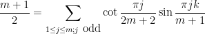
Theorem 1 (Optimal bound for sawtooth inequality) Let.
In particular, we have
- (i) If
for some natural number
.
- (ii) If
for some natural number
.
as
We establish this bound through duality. Indeed, suppose we could find non-negative coefficients 
 . Integrating this against an arbitrary probability measure , we would conclude
 by selecting suitable candidate measures and computing the means
  . The theory of linear programming duality tells us that this method must give us the optimal bound, but one has to locate the optimal measure and optimal weights . This we were able to do by first doing some extensive numerics to discover these weights and measures for small values of , and then doing some educated guesswork to extrapolate these examples to the general case, and then to verify the required inequalities. In case (i) the situation is particularly simple, as one can take to be the discrete measure that assigns a probability
  to the numbers
  and the remaining probability of
  to
to  , while the optimal weighted inequality (1) turns out to be
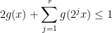
After solving the sawtooth problem, we became interested in the analogous question for the sine function, that is to say what is the best bound 
 Fourier coefficients of . To our knowledge this quantity has not previously been studied in the Fourier analysis literature. By adopting a similar approach as for the sawtooth problem, we were able to compute this quantity exactly also:
Theorem 2 For anyIn particular,
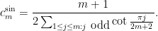
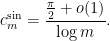
Interestingly, a closely related cotangent sum recently appeared in this MathOverflow post. Verifying the lower bound on 


 , first posed by Eisenstein in 1844 and proved by Stern in 1861. The upper bound arises from establishing the trigonometric inequality
 , which to our knowledge is new; the left-hand side has a Fourier-analytic intepretation as convolving the Fejér kernel with a certain discretized square wave function, and this interpretation is used heavily in our proof of the inequality.
In the modern theory of higher order Fourier analysis, a key role are played by the Gowers uniformity norms 


 denotes complex conjugation, and then on any discrete interval
 ![{[N] = \{1,\dots,N\}}](https://s0.wp.com/latex.php?latex=%7B%5BN%5D+%3D+%5C%7B1%2C%5Cdots%2CN%5C%7D%7D&bg=ffffff&fg=000000&s=0&c=20201002) and any function
and any function ![{f: [N] \rightarrow {\bf C}}](https://s0.wp.com/latex.php?latex=%7Bf%3A+%5BN%5D+%5Crightarrow+%7B%5Cbf+C%7D%7D&bg=ffffff&fg=000000&s=0&c=20201002) we can then define the (normalised) Gowers norm
we can then define the (normalised) Gowers norm ![\displaystyle \|f\|_{U^k([N])} := \| f 1_{[N]} \|_{\tilde U^k({\bf Z})} / \|1_{[N]} \|_{\tilde U^k({\bf Z})}](https://s0.wp.com/latex.php?latex=%5Cdisplaystyle++%5C%7Cf%5C%7C_%7BU%5Ek%28%5BN%5D%29%7D+%3A%3D+%5C%7C+f+1_%7B%5BN%5D%7D+%5C%7C_%7B%5Ctilde+U%5Ek%28%7B%5Cbf+Z%7D%29%7D+%2F+%5C%7C1_%7B%5BN%5D%7D+%5C%7C_%7B%5Ctilde+U%5Ek%28%7B%5Cbf+Z%7D%29%7D&bg=ffffff&fg=000000&s=0&c=20201002)
![{f 1_{[N]}: {\bf Z} \rightarrow {\bf C}}](https://s0.wp.com/latex.php?latex=%7Bf+1_%7B%5BN%5D%7D%3A+%7B%5Cbf+Z%7D+%5Crightarrow+%7B%5Cbf+C%7D%7D&bg=ffffff&fg=000000&s=0&c=20201002) is the extension of by zero to all of
is the extension of by zero to all of  . Thus for instance
 ![\displaystyle \|f\|_{U^1([N])} = |\mathop{\bf E}_{n \in [N]} f(n)|](https://s0.wp.com/latex.php?latex=%5Cdisplaystyle++%5C%7Cf%5C%7C_%7BU%5E1%28%5BN%5D%29%7D+%3D+%7C%5Cmathop%7B%5Cbf+E%7D_%7Bn+%5Cin+%5BN%5D%7D+f%28n%29%7C&bg=ffffff&fg=000000&s=0&c=20201002)
![{\| \|_{U^1([N])}}](https://s0.wp.com/latex.php?latex=%7B%5C%7C+%5C%7C_%7BU%5E1%28%5BN%5D%29%7D%7D&bg=ffffff&fg=000000&s=0&c=20201002) a seminorm rather than a norm), and one can calculate
a seminorm rather than a norm), and one can calculate ![\displaystyle \|f\|_{U^2([N])} \asymp (N \int_0^1 |\mathop{\bf E}_{n \in [N]} f(n) e(-\alpha n)|^4\ d\alpha)^{1/4} \ \ \ \ \ (1)](https://s0.wp.com/latex.php?latex=%5Cdisplaystyle++%5C%7Cf%5C%7C_%7BU%5E2%28%5BN%5D%29%7D+%5Casymp+%28N+%5Cint_0%5E1+%7C%5Cmathop%7B%5Cbf+E%7D_%7Bn+%5Cin+%5BN%5D%7D+f%28n%29+e%28-%5Calpha+n%29%7C%5E4%5C+d%5Calpha%29%5E%7B1%2F4%7D+%5C+%5C+%5C+%5C+%5C+%281%29&bg=ffffff&fg=000000&s=0&c=20201002)
 , and we use the averaging notation
  .
.
The significance of the Gowers norms is that they control other multilinear forms that show up in additive combinatorics. Given any polynomials 
![{f_1,\dots,f_m: [N] \rightarrow {\bf C}}](https://s0.wp.com/latex.php?latex=%7Bf_1%2C%5Cdots%2Cf_m%3A+%5BN%5D+%5Crightarrow+%7B%5Cbf+C%7D%7D&bg=ffffff&fg=000000&s=0&c=20201002)
![\displaystyle \Lambda^{P_1,\dots,P_m}(f_1,\dots,f_m) := \sum_{n \in {\bf Z}^d} \prod_{j=1}^m f_j 1_{[N]}(P_j(n)) / \sum_{n \in {\bf Z}^d} \prod_{j=1}^m 1_{[N]}(P_j(n))](https://s0.wp.com/latex.php?latex=%5Cdisplaystyle++%5CLambda%5E%7BP_1%2C%5Cdots%2CP_m%7D%28f_1%2C%5Cdots%2Cf_m%29+%3A%3D+%5Csum_%7Bn+%5Cin+%7B%5Cbf+Z%7D%5Ed%7D+%5Cprod_%7Bj%3D1%7D%5Em+f_j+1_%7B%5BN%5D%7D%28P_j%28n%29%29+%2F+%5Csum_%7Bn+%5Cin+%7B%5Cbf+Z%7D%5Ed%7D+%5Cprod_%7Bj%3D1%7D%5Em+1_%7B%5BN%5D%7D%28P_j%28n%29%29&bg=ffffff&fg=000000&s=0&c=20201002)
![\displaystyle \Lambda^{\mathrm{n}}(f) = \mathop{\bf E}_{n \in [N]} f(n)](https://s0.wp.com/latex.php?latex=%5Cdisplaystyle++%5CLambda%5E%7B%5Cmathrm%7Bn%7D%7D%28f%29+%3D+%5Cmathop%7B%5Cbf+E%7D_%7Bn+%5Cin+%5BN%5D%7D+f%28n%29&bg=ffffff&fg=000000&s=0&c=20201002)
![\displaystyle \Lambda^{\mathrm{n}, \mathrm{n}+\mathrm{r}}(f,g) = (\mathop{\bf E}_{n \in [N]} f(n)) (\mathop{\bf E}_{n \in [N]} g(n))](https://s0.wp.com/latex.php?latex=%5Cdisplaystyle++%5CLambda%5E%7B%5Cmathrm%7Bn%7D%2C+%5Cmathrm%7Bn%7D%2B%5Cmathrm%7Br%7D%7D%28f%2Cg%29+%3D+%28%5Cmathop%7B%5Cbf+E%7D_%7Bn+%5Cin+%5BN%5D%7D+f%28n%29%29+%28%5Cmathop%7B%5Cbf+E%7D_%7Bn+%5Cin+%5BN%5D%7D+g%28n%29%29&bg=ffffff&fg=000000&s=0&c=20201002)
![\displaystyle \Lambda^{\mathrm{n}, \mathrm{n}+\mathrm{r}, \mathrm{n}+2\mathrm{r}}(f,g,h) \asymp \mathop{\bf E}_{n \in [N]} \mathop{\bf E}_{r \in [-N,N]} f(n) g(n+r) h(n+2r)](https://s0.wp.com/latex.php?latex=%5Cdisplaystyle++%5CLambda%5E%7B%5Cmathrm%7Bn%7D%2C+%5Cmathrm%7Bn%7D%2B%5Cmathrm%7Br%7D%2C+%5Cmathrm%7Bn%7D%2B2%5Cmathrm%7Br%7D%7D%28f%2Cg%2Ch%29+%5Casymp+%5Cmathop%7B%5Cbf+E%7D_%7Bn+%5Cin+%5BN%5D%7D+%5Cmathop%7B%5Cbf+E%7D_%7Br+%5Cin+%5B-N%2CN%5D%7D+f%28n%29+g%28n%2Br%29+h%28n%2B2r%29&bg=ffffff&fg=000000&s=0&c=20201002)
![\displaystyle \Lambda^{\mathrm{n}, \mathrm{n}+\mathrm{r}, \mathrm{n}+\mathrm{r}^2}(f,g,h) \asymp \mathop{\bf E}_{n \in [N]} \mathop{\bf E}_{r \in [-N^{1/2},N^{1/2}]} f(n) g(n+r) h(n+r^2)](https://s0.wp.com/latex.php?latex=%5Cdisplaystyle++%5CLambda%5E%7B%5Cmathrm%7Bn%7D%2C+%5Cmathrm%7Bn%7D%2B%5Cmathrm%7Br%7D%2C+%5Cmathrm%7Bn%7D%2B%5Cmathrm%7Br%7D%5E2%7D%28f%2Cg%2Ch%29+%5Casymp+%5Cmathop%7B%5Cbf+E%7D_%7Bn+%5Cin+%5BN%5D%7D+%5Cmathop%7B%5Cbf+E%7D_%7Br+%5Cin+%5B-N%5E%7B1%2F2%7D%2CN%5E%7B1%2F2%7D%5D%7D+f%28n%29+g%28n%2Br%29+h%28n%2Br%5E2%29&bg=ffffff&fg=000000&s=0&c=20201002)
 as formal (indeterminate) variables, and
 ![{f,g,h: [N] \rightarrow {\bf C}}](https://s0.wp.com/latex.php?latex=%7Bf%2Cg%2Ch%3A+%5BN%5D+%5Crightarrow+%7B%5Cbf+C%7D%7D&bg=ffffff&fg=000000&s=0&c=20201002) are understood to be extended by zero to all of . These forms are used to count patterns in various sets; for instance, the quantity
are understood to be extended by zero to all of . These forms are used to count patterns in various sets; for instance, the quantity  is closely related to the number of length three arithmetic progressions contained in . Let us informally say that a form
  is controlled by the
 ![{U^k[N]}](https://s0.wp.com/latex.php?latex=%7BU%5Ek%5BN%5D%7D&bg=ffffff&fg=000000&s=0&c=20201002) norm if the form is small whenever are -bounded functions with at least one of the
norm if the form is small whenever are -bounded functions with at least one of the  small in norm. This definition was made more precise by Gowers and Wolf, who then defined the true complexity of a form
  to be the least
  such that is controlled by the
 ![{U^{s+1}[N]}](https://s0.wp.com/latex.php?latex=%7BU%5E%7Bs%2B1%7D%5BN%5D%7D&bg=ffffff&fg=000000&s=0&c=20201002) norm. For instance,
norm. For instance,
-
and
have true complexity
;
-
has true complexity
-
has true complexity
- The form
(which among other things could be used to count twin primes) has infinite true complexity (which is quite unfortunate for applications).
or less are amenable to being studied by classical Fourier analytic tools (the Hardy-Littlewood circle method); patterns of higher complexity can be handled (in principle, at least) by the methods of higher order Fourier analysis; and patterns of infinite complexity are out of range of both methods and are generally quite difficult to study. See these recent slides of myself (or this video of the lecture) for some further discussion.
Gowers and Wolf formulated a conjecture on what this complexity should be, at least for linear polynomials 
The 
![\displaystyle \Lambda^{2\mathrm{n}}(f) = \mathop{\bf E}_{n \in [N], \hbox{ even}} f(n)](https://s0.wp.com/latex.php?latex=%5Cdisplaystyle++%5CLambda%5E%7B2%5Cmathrm%7Bn%7D%7D%28f%29+%3D+%5Cmathop%7B%5Cbf+E%7D_%7Bn+%5Cin+%5BN%5D%2C+%5Chbox%7B+even%7D%7D+f%28n%29&bg=ffffff&fg=000000&s=0&c=20201002)
![{U^1[N]}](https://s0.wp.com/latex.php?latex=%7BU%5E1%5BN%5D%7D&bg=ffffff&fg=000000&s=0&c=20201002) semi-norm: it is perfectly possible for a -bounded function to even have vanishing
semi-norm: it is perfectly possible for a -bounded function to even have vanishing ![{U^1([N])}](https://s0.wp.com/latex.php?latex=%7BU%5E1%28%5BN%5D%29%7D&bg=ffffff&fg=000000&s=0&c=20201002) norm but have large value of
norm but have large value of  (consider for instance the parity function
  ).
).
Because of this, I propose inserting an additional norm in the Gowers uniformity norm hierarchy between the 

![\displaystyle \| f\|_{U^{1^+}[N]} := \frac{1}{N} \sup_P |\sum_{n \in P} f(n)| = \sup_P | \mathop{\bf E}_{n \in [N]} f 1_P(n)|](https://s0.wp.com/latex.php?latex=%5Cdisplaystyle++%5C%7C+f%5C%7C_%7BU%5E%7B1%5E%2B%7D%5BN%5D%7D+%3A%3D+%5Cfrac%7B1%7D%7BN%7D+%5Csup_P+%7C%5Csum_%7Bn+%5Cin+P%7D+f%28n%29%7C+%3D+%5Csup_P+%7C+%5Cmathop%7B%5Cbf+E%7D_%7Bn+%5Cin+%5BN%5D%7D+f+1_P%28n%29%7C&bg=ffffff&fg=000000&s=0&c=20201002) ranges over all arithmetic progressions in
ranges over all arithmetic progressions in ![{[N]}](https://s0.wp.com/latex.php?latex=%7B%5BN%5D%7D&bg=ffffff&fg=000000&s=0&c=20201002) . This can easily be seen to be a norm on functions that controls the norm. It is also basically controlled by the
. This can easily be seen to be a norm on functions that controls the norm. It is also basically controlled by the ![{U^2[N]}](https://s0.wp.com/latex.php?latex=%7BU%5E2%5BN%5D%7D&bg=ffffff&fg=000000&s=0&c=20201002) norm for -bounded functions ; indeed, if is an arithmetic progression in of some spacing
norm for -bounded functions ; indeed, if is an arithmetic progression in of some spacing  , then we can write as the intersection of an interval
  with a residue class modulo
  , and from Fourier expansion we have
 ![\displaystyle \mathop{\bf E}_{n \in [N]} f 1_P(n) \ll \sup_\alpha |\mathop{\bf E}_{n \in [N]} f 1_I(n) e(\alpha n)|.](https://s0.wp.com/latex.php?latex=%5Cdisplaystyle++%5Cmathop%7B%5Cbf+E%7D_%7Bn+%5Cin+%5BN%5D%7D+f+1_P%28n%29+%5Cll+%5Csup_%5Calpha+%7C%5Cmathop%7B%5Cbf+E%7D_%7Bn+%5Cin+%5BN%5D%7D+f+1_I%28n%29+e%28%5Calpha+n%29%7C.&bg=ffffff&fg=000000&s=0&c=20201002)
 be a standard bump function supported on
 ![{[-1,1]}](https://s0.wp.com/latex.php?latex=%7B%5B-1%2C1%5D%7D&bg=ffffff&fg=000000&s=0&c=20201002) with total mass and
with total mass and  is a parameter then
 ![\displaystyle \mathop{\bf E}_{n \in [N]} f 1_I(n) e(\alpha n)](https://s0.wp.com/latex.php?latex=%5Cdisplaystyle++%5Cmathop%7B%5Cbf+E%7D_%7Bn+%5Cin+%5BN%5D%7D+f+1_I%28n%29+e%28%5Calpha+n%29+&bg=ffffff&fg=000000&s=0&c=20201002)
![\displaystyle \ll |\mathop{\bf E}_{n \in [-N,2N]; h, k \in [-N,N]} \frac{1}{\delta} \psi(\frac{h}{\delta N})](https://s0.wp.com/latex.php?latex=%5Cdisplaystyle+%5Cll+%7C%5Cmathop%7B%5Cbf+E%7D_%7Bn+%5Cin+%5B-N%2C2N%5D%3B+h%2C+k+%5Cin+%5B-N%2CN%5D%7D+%5Cfrac%7B1%7D%7B%5Cdelta%7D+%5Cpsi%28%5Cfrac%7Bh%7D%7B%5Cdelta+N%7D%29&bg=ffffff&fg=000000&s=0&c=20201002)

![\displaystyle \ll |\mathop{\bf E}_{n \in [-N,2N]; h, k \in [-N,N]} \frac{1}{\delta} \psi(\frac{h}{\delta N}) 1_I(n+k) f(n+h+k) e(\alpha(n+h+k))|](https://s0.wp.com/latex.php?latex=%5Cdisplaystyle++%5Cll+%7C%5Cmathop%7B%5Cbf+E%7D_%7Bn+%5Cin+%5B-N%2C2N%5D%3B+h%2C+k+%5Cin+%5B-N%2CN%5D%7D+%5Cfrac%7B1%7D%7B%5Cdelta%7D+%5Cpsi%28%5Cfrac%7Bh%7D%7B%5Cdelta+N%7D%29+1_I%28n%2Bk%29+f%28n%2Bh%2Bk%29+e%28%5Calpha%28n%2Bh%2Bk%29%29%7C+&bg=ffffff&fg=000000&s=0&c=20201002)
 by zero outside of ), as can be seen by using the triangle inequality and the estimate
 ![\displaystyle \mathop{\bf E}_{h \in [-N,N]} \frac{1}{\delta} \psi(\frac{h}{\delta N}) 1_I(n+h+k) - \mathop{\bf E}_{h \in [-N,N]} \frac{1}{\delta} \psi(\frac{h}{\delta N}) 1_I(n+k)](https://s0.wp.com/latex.php?latex=%5Cdisplaystyle++%5Cmathop%7B%5Cbf+E%7D_%7Bh+%5Cin+%5B-N%2CN%5D%7D+%5Cfrac%7B1%7D%7B%5Cdelta%7D+%5Cpsi%28%5Cfrac%7Bh%7D%7B%5Cdelta+N%7D%29+1_I%28n%2Bh%2Bk%29+-+%5Cmathop%7B%5Cbf+E%7D_%7Bh+%5Cin+%5B-N%2CN%5D%7D+%5Cfrac%7B1%7D%7B%5Cdelta%7D+%5Cpsi%28%5Cfrac%7Bh%7D%7B%5Cdelta+N%7D%29+1_I%28n%2Bk%29&bg=ffffff&fg=000000&s=0&c=20201002)

 we now have
 ![\displaystyle \mathop{\bf E}_{n \in [N]} f 1_P(n) \ll \frac{1}{\delta} \sup_{\alpha,\beta} |\mathop{\bf E}_{n \in [N]; h, k \in [-N,N]} e(\beta h + \alpha (n+h+k))](https://s0.wp.com/latex.php?latex=%5Cdisplaystyle++%5Cmathop%7B%5Cbf+E%7D_%7Bn+%5Cin+%5BN%5D%7D+f+1_P%28n%29+%5Cll+%5Cfrac%7B1%7D%7B%5Cdelta%7D+%5Csup_%7B%5Calpha%2C%5Cbeta%7D+%7C%5Cmathop%7B%5Cbf+E%7D_%7Bn+%5Cin+%5BN%5D%3B+h%2C+k+%5Cin+%5B-N%2CN%5D%7D+e%28%5Cbeta+h+%2B+%5Calpha+%28n%2Bh%2Bk%29%29+&bg=ffffff&fg=000000&s=0&c=20201002)

 as a linear combination of
  and using the Gowers–Cauchy–Schwarz inequality, we conclude
 ![\displaystyle \mathop{\bf E}_{n \in [N]} f 1_P(n) \ll \frac{1}{\delta} \|f\|_{U^2([N])} + \delta](https://s0.wp.com/latex.php?latex=%5Cdisplaystyle++%5Cmathop%7B%5Cbf+E%7D_%7Bn+%5Cin+%5BN%5D%7D+f+1_P%28n%29+%5Cll+%5Cfrac%7B1%7D%7B%5Cdelta%7D+%5C%7Cf%5C%7C_%7BU%5E2%28%5BN%5D%29%7D+%2B+%5Cdelta&bg=ffffff&fg=000000&s=0&c=20201002)
 we have
 ![\displaystyle \| f\|_{U^{1^+}[N]} \ll \|f\|_{U^2[N]}^{1/2}.](https://s0.wp.com/latex.php?latex=%5Cdisplaystyle++%5C%7C+f%5C%7C_%7BU%5E%7B1%5E%2B%7D%5BN%5D%7D+%5Cll+%5C%7Cf%5C%7C_%7BU%5E2%5BN%5D%7D%5E%7B1%2F2%7D.&bg=ffffff&fg=000000&s=0&c=20201002) norm (but not ) would then have their true complexity adjusted to
norm (but not ) would then have their true complexity adjusted to  with this insertion.
The 


The well known inverse theorem for the 


![\displaystyle |\mathop{\bf E}_{n \in [N]} f(n) e(-\alpha n)| \gg \eta^2;](https://s0.wp.com/latex.php?latex=%5Cdisplaystyle++%7C%5Cmathop%7B%5Cbf+E%7D_%7Bn+%5Cin+%5BN%5D%7D+f%28n%29+e%28-%5Calpha+n%29%7C+%5Cgg+%5Ceta%5E2%3B&bg=ffffff&fg=000000&s=0&c=20201002)
![\displaystyle |\mathop{\bf E}_{n \in [N]} f(n) e(-\alpha n)| \ll \|f\|_{U^2[N]}.](https://s0.wp.com/latex.php?latex=%5Cdisplaystyle++%7C%5Cmathop%7B%5Cbf+E%7D_%7Bn+%5Cin+%5BN%5D%7D+f%28n%29+e%28-%5Calpha+n%29%7C+%5Cll+%5C%7Cf%5C%7C_%7BU%5E2%5BN%5D%7D.&bg=ffffff&fg=000000&s=0&c=20201002)
For
![\displaystyle |\mathop{\bf E}_{n \in [N]} f(n)| \geq \eta.](https://s0.wp.com/latex.php?latex=%5Cdisplaystyle++%7C%5Cmathop%7B%5Cbf+E%7D_%7Bn+%5Cin+%5BN%5D%7D+f%28n%29%7C+%5Cgeq+%5Ceta.&bg=ffffff&fg=000000&s=0&c=20201002)
 appearing in the inverse theorem can be taken to be zero when working instead with the norm.
For ![{\|f\|_{U^{1^+}[N]} \geq \eta}](https://s0.wp.com/latex.php?latex=%7B%5C%7Cf%5C%7C_%7BU%5E%7B1%5E%2B%7D%5BN%5D%7D+%5Cgeq+%5Ceta%7D&bg=ffffff&fg=000000&s=0&c=20201002)
![\displaystyle |\mathop{\bf E}_{n \in [N]} 1_P(n) f(n)| \geq \eta](https://s0.wp.com/latex.php?latex=%5Cdisplaystyle++%7C%5Cmathop%7B%5Cbf+E%7D_%7Bn+%5Cin+%5BN%5D%7D+1_P%28n%29+f%28n%29%7C+%5Cgeq+%5Ceta&bg=ffffff&fg=000000&s=0&c=20201002) . This forces the spacing of this progression to be
. This forces the spacing of this progression to be  . We write the above inequality as
 ![\displaystyle |\mathop{\bf E}_{n \in [N]} 1_{n=b\ (q)} 1_I(n) f(n)| \geq \eta](https://s0.wp.com/latex.php?latex=%5Cdisplaystyle++%7C%5Cmathop%7B%5Cbf+E%7D_%7Bn+%5Cin+%5BN%5D%7D+1_%7Bn%3Db%5C+%28q%29%7D+1_I%28n%29+f%28n%29%7C+%5Cgeq+%5Ceta&bg=ffffff&fg=000000&s=0&c=20201002)
 and some interval . By Fourier expansion and the triangle inequality we then have
 ![\displaystyle |\mathop{\bf E}_{n \in [N]} e(-an/q) 1_I(n) f(n)| \geq \eta](https://s0.wp.com/latex.php?latex=%5Cdisplaystyle++%7C%5Cmathop%7B%5Cbf+E%7D_%7Bn+%5Cin+%5BN%5D%7D+e%28-an%2Fq%29+1_I%28n%29+f%28n%29%7C+%5Cgeq+%5Ceta&bg=ffffff&fg=000000&s=0&c=20201002)
 . Convolving
  by
by  for a small multiple of and a Schwartz function of unit mass with Fourier transform supported on , we have
 ![\displaystyle |\mathop{\bf E}_{n \in [N]} e(-an/q) (1_I * \psi_\delta)(n) f(n)| \gg \eta.](https://s0.wp.com/latex.php?latex=%5Cdisplaystyle++%7C%5Cmathop%7B%5Cbf+E%7D_%7Bn+%5Cin+%5BN%5D%7D+e%28-an%2Fq%29+%281_I+%2A+%5Cpsi_%5Cdelta%29%28n%29+f%28n%29%7C+%5Cgg+%5Ceta.&bg=ffffff&fg=000000&s=0&c=20201002)
 of
of  is bounded by
  and supported on
 ![{[-\frac{1}{\delta N},\frac{1}{\delta N}]}](https://s0.wp.com/latex.php?latex=%7B%5B-%5Cfrac%7B1%7D%7B%5Cdelta+N%7D%2C%5Cfrac%7B1%7D%7B%5Cdelta+N%7D%5D%7D&bg=ffffff&fg=000000&s=0&c=20201002) , thus by Fourier expansion and the triangle inequality we have
, thus by Fourier expansion and the triangle inequality we have ![\displaystyle |\mathop{\bf E}_{n \in [N]} e(-an/q) e(-\xi n) f(n)| \gg \eta^2](https://s0.wp.com/latex.php?latex=%5Cdisplaystyle++%7C%5Cmathop%7B%5Cbf+E%7D_%7Bn+%5Cin+%5BN%5D%7D+e%28-an%2Fq%29+e%28-%5Cxi+n%29+f%28n%29%7C+%5Cgg+%5Ceta%5E2&bg=ffffff&fg=000000&s=0&c=20201002)
![{\xi \in [-\frac{1}{\delta N},\frac{1}{\delta N}]}](https://s0.wp.com/latex.php?latex=%7B%5Cxi+%5Cin+%5B-%5Cfrac%7B1%7D%7B%5Cdelta+N%7D%2C%5Cfrac%7B1%7D%7B%5Cdelta+N%7D%5D%7D&bg=ffffff&fg=000000&s=0&c=20201002) , so in particular
, so in particular  . Thus we have
 ![\displaystyle |\mathop{\bf E}_{n \in [N]} f(n) e(-\alpha n)| \gg \eta^2 \ \ \ \ \ (2)](https://s0.wp.com/latex.php?latex=%5Cdisplaystyle++%7C%5Cmathop%7B%5Cbf+E%7D_%7Bn+%5Cin+%5BN%5D%7D+f%28n%29+e%28-%5Calpha+n%29%7C+%5Cgg+%5Ceta%5E2+%5C+%5C+%5C+%5C+%5C+%282%29&bg=ffffff&fg=000000&s=0&c=20201002) of the major arc form
of the major arc form  with
with  . Conversely, for of this form, some routine summation by parts gives the bound
 ![\displaystyle |\mathop{\bf E}_{n \in [N]} f(n) e(-\alpha n)| \ll \frac{q}{\eta} \|f\|_{U^{1^+}[N]} \ll \frac{1}{\eta^2} \|f\|_{U^{1^+}[N]}](https://s0.wp.com/latex.php?latex=%5Cdisplaystyle++%7C%5Cmathop%7B%5Cbf+E%7D_%7Bn+%5Cin+%5BN%5D%7D+f%28n%29+e%28-%5Calpha+n%29%7C+%5Cll+%5Cfrac%7Bq%7D%7B%5Ceta%7D+%5C%7Cf%5C%7C_%7BU%5E%7B1%5E%2B%7D%5BN%5D%7D+%5Cll+%5Cfrac%7B1%7D%7B%5Ceta%5E2%7D+%5C%7Cf%5C%7C_%7BU%5E%7B1%5E%2B%7D%5BN%5D%7D&bg=ffffff&fg=000000&s=0&c=20201002) -bounded then one must have
-bounded then one must have ![{\|f\|_{U^{1^+}[N]} \gg \eta^4}](https://s0.wp.com/latex.php?latex=%7B%5C%7Cf%5C%7C_%7BU%5E%7B1%5E%2B%7D%5BN%5D%7D+%5Cgg+%5Ceta%5E4%7D&bg=ffffff&fg=000000&s=0&c=20201002) .
.
Here is a diagram showing some of the control relationships between various Gowers norms, multilinear forms, and duals of classes ![{\| f \|_{{\mathcal F}^*} := \sup_{\phi \in {\mathcal F}} \mathop{\bf E}_{n \in[N]} f(n) \overline{\phi(n)}}](https://s0.wp.com/latex.php?latex=%7B%5C%7C+f+%5C%7C_%7B%7B%5Cmathcal+F%7D%5E%2A%7D+%3A%3D+%5Csup_%7B%5Cphi+%5Cin+%7B%5Cmathcal+F%7D%7D+%5Cmathop%7B%5Cbf+E%7D_%7Bn+%5Cin%5BN%5D%7D+f%28n%29+%5Coverline%7B%5Cphi%28n%29%7D%7D&bg=ffffff&fg=000000&s=0&c=20201002)

Here I have included the three classes of functions that one can choose from for the 
The Gowers norms have counterparts for measure-preserving systems 


![\displaystyle \|f\|_{U^1(X)} := \lim_{N \rightarrow \infty} \int_X |\mathop{\bf E}_{n \in [N]} T^n f|\ d\mu](https://s0.wp.com/latex.php?latex=%5Cdisplaystyle++%5C%7Cf%5C%7C_%7BU%5E1%28X%29%7D+%3A%3D+%5Clim_%7BN+%5Crightarrow+%5Cinfty%7D+%5Cint_X+%7C%5Cmathop%7B%5Cbf+E%7D_%7Bn+%5Cin+%5BN%5D%7D+T%5En+f%7C%5C+d%5Cmu&bg=ffffff&fg=000000&s=0&c=20201002) norm can be defined as
norm can be defined as ![\displaystyle \|f\|_{U^2(X)}^4 := \lim_{N \rightarrow \infty} \mathop{\bf E}_{n \in [N]} \| T^n f \overline{f} \|_{U^1(X)}^2.](https://s0.wp.com/latex.php?latex=%5Cdisplaystyle++%5C%7Cf%5C%7C_%7BU%5E2%28X%29%7D%5E4+%3A%3D+%5Clim_%7BN+%5Crightarrow+%5Cinfty%7D+%5Cmathop%7B%5Cbf+E%7D_%7Bn+%5Cin+%5BN%5D%7D+%5C%7C+T%5En+f+%5Coverline%7Bf%7D+%5C%7C_%7BU%5E1%28X%29%7D%5E2.&bg=ffffff&fg=000000&s=0&c=20201002) seminorm is orthogonal to the invariant factor
seminorm is orthogonal to the invariant factor  (generated by the (almost everywhere) invariant measurable subsets of ) in the sense that a function has vanishing seminorm if and only if it is orthogonal to all -measurable (bounded) functions. Similarly, the
  norm is orthogonal to the Kronecker factor
  , generated by the eigenfunctions of (that is to say, those obeying an identity
  for some -invariant
  ); for ergodic systems, it is the largest factor isomorphic to rotation on a compact abelian group. In analogy to the Gowers
 ![{U^{1^+}[N]}](https://s0.wp.com/latex.php?latex=%7BU%5E%7B1%5E%2B%7D%5BN%5D%7D&bg=ffffff&fg=000000&s=0&c=20201002) norm, one can then define the Host-Kra
norm, one can then define the Host-Kra  seminorm by
 ![\displaystyle \|f\|_{U^{1^+}(X)} := \sup_{q \geq 1} \frac{1}{q} \lim_{N \rightarrow \infty} \int_X |\mathop{\bf E}_{n \in [N]} T^{qn} f|\ d\mu;](https://s0.wp.com/latex.php?latex=%5Cdisplaystyle++%5C%7Cf%5C%7C_%7BU%5E%7B1%5E%2B%7D%28X%29%7D+%3A%3D+%5Csup_%7Bq+%5Cgeq+1%7D+%5Cfrac%7B1%7D%7Bq%7D+%5Clim_%7BN+%5Crightarrow+%5Cinfty%7D+%5Cint_X+%7C%5Cmathop%7B%5Cbf+E%7D_%7Bn+%5Cin+%5BN%5D%7D+T%5E%7Bqn%7D+f%7C%5C+d%5Cmu%3B&bg=ffffff&fg=000000&s=0&c=20201002)
 , generated by the periodic sets of (or equivalently, by those eigenfunctions whose eigenvalue is a root of unity); for ergodic systems, it is the largest factor isomorphic to rotation on a profinite abelian group.

Recent Comments