
You are currently browsing the category archive for the ‘math.MG’ category.
Jan Grebik, Rachel Greenfeld, Vaclav Rozhon and I have just uploaded to the arXiv our preprint “Measurable tilings by abelian group actions“. This paper is related to an earlier paper of Rachel Greenfeld and myself concerning tilings of lattices 


If 


![{A = [0,1/2]^2 \hbox{ mod } {\bf Z}^2}](https://s0.wp.com/latex.php?latex=%7BA+%3D+%5B0%2C1%2F2%5D%5E2+%5Chbox%7B+mod+%7D+%7B%5Cbf+Z%7D%5E2%7D&bg=ffffff&fg=000000&s=0&c=20201002)

- By modifying arguments from previous papers (including the one with Greenfeld mentioned above), we can establish the following “dilation lemma”: a measurable tiling
, whenever
is an integer coprime to all primes up to the cardinality
of
- By averaging the above dilation lemma, we can also establish a “structure theorem” that decomposes the indicator function
of
- By applying this structure theorem, we can show that all measurable tilings
of the one-dimensional torus
are rational, in the sense that
. This answers a recent conjecture of Conley, Grebik, and Pikhurko; we also give an alternate proof of this conjecture using some previous results of Lagarias and Wang.
- For tilings
of higher-dimensional tori, the tiling need not be rational. However, we can show that we can “slide” the tiling to be rational by giving each translate
of
, and for every time
, the translates
still form a partition of
modulo null sets, and at time
the tiling becomes rational. In particular, if a set
- In the two-dimensional case
one can arrange matters so that all the velocities
are parallel. If we furthermore assume that the tile
form a
-invariant subset of the torus.
- Finally, we show that tilings
of a finitely generated discrete group
, with
. (Nonabelian local tilings, for instance of the sphere by rotations, are of interest due to connections with the Banach-Tarski paradox; see the aforementioned paper of Conley, Grebik, and Pikhurko. Unfortunately, our methods seem to break down completely in the nonabelian case.)
I’ve just uploaded to the arXiv my preprint “Perfectly packing a square by squares of nearly harmonic sidelength“. This paper concerns a variant of an old problem of Meir and Moser, who asks whether it is possible to perfectly pack squares of sidelength 


Another direction in which partial progress has been made is to consider instead the problem of packing squares of sidelength 


In this paper we are able to get
Theorem 1 If, and
is sufficiently large depending on
perfectly into a square of area
.
As in previous works, the general strategy is to execute a greedy algorithm, which can be described somewhat incompletely as follows.
- Step 1: Suppose that one has already managed to perfectly pack a square
of area
, together with a further finite collection
of rectangles with disjoint interiors. (Initially, we would have
and
, but these parameter will change over the course of the algorithm.)
- Step 2: Amongst all the rectangles in
of the largest width (defined as the shorter of the two sidelengths of
- Step 3: Pack (as efficiently as one can) squares of sidelength
into
, and decompose the portion of
.
- Step 4: Replace
by
, replace
, and return to Step 1.
The main innovation of this paper is to perform Step 3 somewhat more efficiently than in previous papers.
The above algorithm can get stuck if one reaches a point where one has already packed squares of sidelength 


 of these rectangles is
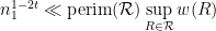 with
with  it would be enough to have the perimeter bound
 . It is here that we now see the critical nature of the exponent : for
  , the amount of perimeter we are permitted to have in the remaining rectangles increases as one progresses with the packing, but for the amount of perimeter one is “budgeted” for stays constant (and for
  the situation is even worse, in that the remaining rectangles should steadily decrease in total perimeter).
In comparison, the perimeter of the squares that one has already packed is equal to

 for large (with the constants blowing up as approaches the critical value of ). In previous algorithms, the total perimeter of the remainder rectangles was basically comparable to the perimeter of the squares already packed, and this is the main reason why the results only worked when was sufficiently far away from . In my paper, I am able to get the perimeter of significantly smaller than the perimeter of the squares already packed, by grouping those squares into lattice-like clusters (of about
  squares arranged in an
  pattern), and sliding the squares in each cluster together to almost entirely eliminate the wasted space between each square, leaving only the space around the cluster as the main source of residual perimeter, which will be comparable to about
  per cluster, as compared to the total perimeter of the squares in the cluster which is comparable to
  . This strategy is perhaps easiest to illustrate with a picture, in which
  squares
  of slowly decreasing sidelength are packed together with relatively little wasted space:

By choosing the parameter 


Given three points 

but are otherwise unconstrained. But if one has four points 

Proposition 1 (Cayley-Menger determinant) If
vanishes.

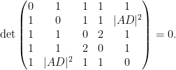
Proof: If we view 


and 

The matrix 


For instance, if we know that 


After some calculation the left-hand side simplifies to 


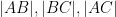
Now suppose that we have four points 

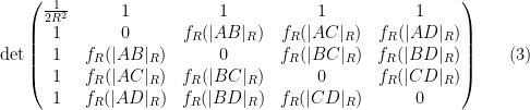
Proposition 2 (Spherical Cayley-Menger determinant) If
, then the spherical Cayley-Menger determinant
vanishes.

Proof: We can assume that the sphere 


Similarly for all the other inner products. Thus the matrix in (2) can be written as 
We can factor 


Just as the Cayley-Menger determinant can be used to test for coplanarity, the spherical Cayley-Menger determinant can be used to test for lying on a sphere of radius 


The left-hand side evaluates to 


The Cayley-Menger and spherical Cayley-Menger determinants look slightly different from each other, but one can transform the latter into something resembling the former by row and column operations. Indeed, the determinant (2) can be rewritten as

and by further row and column operations, this determinant vanishes if and only if the determinant
vanishes, where 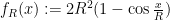


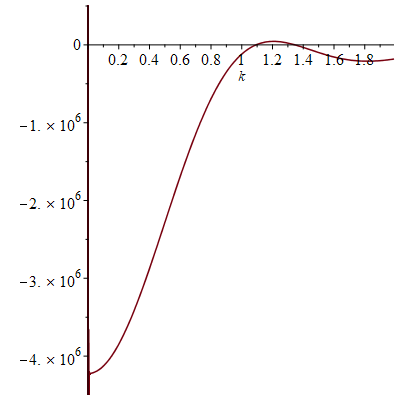
In principle, one can now estimate the radius 


Given that the true radius of the earth was about 


In particular, the determinant does indeed come very close to vanishing when 


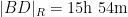
If instead one goes to the flight time calculator and uses flight travel times instead of distances, one now gets the following data (measured in hours):

Assuming that planes travel at about 


Not too surprisingly, this is basically a rescaled version of the previous plot, with vanishing near 
Of course, these two data sets are “cheating” since they come from a model which already presupposes what the radius of the Earth is. But one can input real world flight times between these four cities instead of the above idealised data. Here one runs into the issue that the flight time from


This data is not too far off from the online calculator data, but it does distort the graph slightly (taking 

Now one gets estimates for the radius of the Earth that are off by about a factor of
Given that windspeed should additively affect flight velocity rather than flight time, and the two are inversely proportional to each other, it is more natural to take a harmonic mean rather than an arithmetic mean. This gives the slightly different values


but one still gets essentially the same plot:

So the inaccuracies are presumably coming from some other source. (Note for instance that the true flight time from Tokyo to Dubai is about 

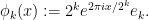
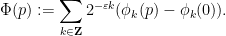
I’ve just uploaded to the arXiv my paper “Embedding the Heisenberg group into a bounded dimensional Euclidean space with optimal distortion“, submitted to Revista Matematica Iberoamericana. This paper concerns the extent to which one can accurately embed the metric structure of the Heisenberg group
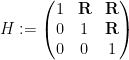
into Euclidean space, which we can write as ![{\{ [x,y,z]: x,y,z \in {\bf R} \}}](https://s0.wp.com/latex.php?latex=%7B%5C%7B+%5Bx%2Cy%2Cz%5D%3A+x%2Cy%2Cz+%5Cin+%7B%5Cbf+R%7D+%5C%7D%7D&bg=ffffff&fg=000000&s=0&c=20201002)
![\displaystyle [x,y,z] := \begin{pmatrix} 1 & x & z \\ 0 & 1 & y \\ 0 & 0 & 1 \end{pmatrix}.](https://s0.wp.com/latex.php?latex=%5Cdisplaystyle+%5Bx%2Cy%2Cz%5D+%3A%3D+%5Cbegin%7Bpmatrix%7D+1+%26+x+%26+z+%5C%5C+0+%26+1+%26+y+%5C%5C+0+%26+0+%26+1+%5Cend%7Bpmatrix%7D.&bg=ffffff&fg=000000&s=0&c=20201002)
Here we give 

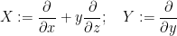
but not from the commutator vector field
![\displaystyle Z := [Y,X] = \frac{\partial}{\partial z}.](https://s0.wp.com/latex.php?latex=%5Cdisplaystyle+Z+%3A%3D+%5BY%2CX%5D+%3D+%5Cfrac%7B%5Cpartial%7D%7B%5Cpartial+z%7D.&bg=ffffff&fg=000000&s=0&c=20201002)
This gives 


On the other hand, if one snowflakes the Heisenberg group by replacing the metric 


Of course, the distortion of this bilipschitz embedding must degenerate in the limit 


The main result of this paper answers this question in the negative:
Theorem 1 There exists an absolute constant
for any
.
To motivate the proof of this theorem, let us first present a bilipschitz map 


where for each 

and 


with the lower bound

at which point one finds that

as desired.
The key here was that each function 


![{\Gamma := \{ [a,b,c]: a,b,c \in {\bf Z} \}}](https://s0.wp.com/latex.php?latex=%7B%5CGamma+%3A%3D+%5C%7B+%5Ba%2Cb%2Cc%5D%3A+a%2Cb%2Cc+%5Cin+%7B%5Cbf+Z%7D+%5C%7D%7D&bg=ffffff&fg=000000&s=0&c=20201002)


where 
![\displaystyle \delta_\lambda([x,y,z]) := [\lambda x, \lambda y, \lambda^2 z],](https://s0.wp.com/latex.php?latex=%5Cdisplaystyle+%5Cdelta_%5Clambda%28%5Bx%2Cy%2Cz%5D%29+%3A%3D+%5B%5Clambda+x%2C+%5Clambda+y%2C+%5Clambda%5E2+z%5D%2C&bg=ffffff&fg=000000&s=0&c=20201002)
then one can repeat the previous arguments to obtain the required bilipschitz bounds

for the function
To adapt this construction to bounded dimension, the main obstruction was the requirement that the
for all 


One can then try to construct the 


We view this as an underdetermined system of differential equations for 


This problem has some formal similarities with the isometric embedding problem (discussed for instance in this previous post), which can be viewed as the problem of solving an equation of the form 


The isometric embedding problem also has the key obstacle that naive attempts to solve the equation 
To motivate this iteration, we first express 

This reveals that one can construct solutions

for 


To get around this obstacle (which also prominently appears when solving (linearisations of) the isometric embedding equation 

where 


We will construct the low-frequency solution 


To perform the deformation of

of (1) when 


As before, if one directly solves the difference equation (5) using a naive application of (2) with 


and then one can solve (5) by solving the system of equations
for 
that one would obtain from naively linearising (3) without exploiting the symmetry of 


Previous set of notes: Notes 1. Next set of notes: Notes 3.
We now leave the topic of Riemann surfaces, and turn now to the (loosely related) topic of conformal mapping (and quasiconformal mapping). Recall that a conformal map 


In previous quarters, we proved a fundamental theorem about this concept, the Riemann mapping theorem:
Theorem 1 (Riemann mapping theorem) Let
that is not all of
.
This theorem was proven in these 246A lecture notes, using an argument of Koebe. At a very high level, one can sketch Koebe’s proof of the Riemann mapping theorem as follows: among all the injective holomorphic maps 


It is a beautiful observation of Thurston that the concept of a conformal mapping has a discrete counterpart, namely the mapping of one circle packing to another. Furthermore, one can run a version of Koebe’s argument (using now a discrete version of Perron’s method) to prove the Riemann mapping theorem through circle packings. In principle, this leads to a mostly elementary approach to conformal geometry, based on extremely classical mathematics that goes all the way back to Apollonius. However, in order to prove the basic existence and uniqueness theorems of circle packing, as well as the convergence to conformal maps in the continuous limit, it seems to be necessary (or at least highly convenient) to use much more modern machinery, including the theory of quasiconformal mapping, and also the Riemann mapping theorem itself (so in particular we are not structuring these notes to provide a completely independent proof of that theorem, though this may well be possible).
To make the above discussion more precise we need some notation.
Definition 2 (Circle packing) A (finite) circle packing is a finite collection
of circles
in the complex numbers indexed by some finite set
, whose interiors are all disjoint (but which are allowed to be tangent to each other), and whose union is connected. The nerve of a circle packing is the finite graph whose vertices
are the centres of the circle packing, with two such centres connected by an edge if the circles are tangent. (In these notes all graphs are undirected, finite and simple, unless otherwise specified.)
It is clear that the nerve of a circle packing is connected and planar, since one can draw the nerve by placing each vertex (tautologically) in its location in the complex plane, and drawing each edge by the line segment between the centres of the circles it connects (this line segment will pass through the point of tangency of the two circles). Later in these notes we will also have to consider some infinite circle packings, most notably the infinite regular hexagonal circle packing.
The first basic theorem in the subject is the following converse statement:
Theorem 3 (Circle packing theorem) Every connected planar graph is the nerve of a circle packing.
Among other things, the circle packing theorem thus implies as a corollary Fáry’s theorem that every planar graph can be drawn using straight lines.
Of course, there can be multiple circle packings associated to a given connected planar graph; indeed, since reflections across a line and Möbius transformations map circles to circles (or lines), they will map circle packings to circle packings (unless one or more of the circles is sent to a line). It turns out that once one adds enough edges to the planar graph, the circle packing is otherwise rigid:
Theorem 4 (Koebe-Andreev-Thurston theorem) If a connected planar graph is maximal (i.e., no further edge can be added to it without destroying planarity), then the circle packing given by the above theorem is unique up to reflections and Möbius transformations.
Exercise 5 Let
vertices. Show that the following are equivalent:
- (i)
- (ii)
edges.
- (iii) Every drawing
- (iv) At least one drawing
(Hint: you may use without proof Euler’s formula
for planar graphs, where
Thurston conjectured that circle packings can be used to approximate the conformal map arising in the Riemann mapping theorem. Here is an informal statement:
Conjecture 6 (Informal Thurston conjecture) Let
to the origin and
to a positive real. For any small
, let
be the portion of the regular hexagonal circle packing by circles of radius
be an circle packing of
defined on the subset
of
is zero and
is a positive real. Then
converges to
A rigorous version of this conjecture was proven by Rodin and Sullivan. Besides some elementary geometric lemmas (regarding the relative sizes of various configurations of tangent circles), the main ingredients are a rigidity result for the regular hexagonal circle packing, and the theory of quasiconformal maps. Quasiconformal maps are what seem on the surface to be a very broad generalisation of the notion of a conformal map. Informally, conformal maps take infinitesimal circles to infinitesimal circles, whereas quasiconformal maps take infinitesimal circles to infinitesimal ellipses of bounded eccentricity. In terms of Wirtinger derivatives, conformal maps obey the Cauchy-Riemann equation 
The Polymath14 online collaboration has uploaded to the arXiv its paper “Homogeneous length functions on groups“, submitted to Algebra & Number Theory. The paper completely classifies homogeneous length functions 


The proof is based on repeated use of the homogeneous length function axioms, combined with elementary identities of commutators, to obtain increasingly good bounds on quantities such as ![{\|[x,y]\|}](https://s0.wp.com/latex.php?latex=%7B%5C%7C%5Bx%2Cy%5D%5C%7C%7D&bg=ffffff&fg=000000&s=0&c=20201002)
As there are now a large number of comments on the previous post on this project, this post will also serve as the new thread for any final discussion of this project as it winds down.
In the tradition of “Polymath projects“, the problem posed in the previous two blog posts has now been solved, thanks to the cumulative effect of many small contributions by many participants (including, but not limited to, Sean Eberhard, Tobias Fritz, Siddharta Gadgil, Tobias Hartnick, Chris Jerdonek, Apoorva Khare, Antonio Machiavelo, Pace Nielsen, Andy Putman, Will Sawin, Alexander Shamov, Lior Silberman, and David Speyer). In this post I’ll write down a streamlined resolution, eliding a number of important but ultimately removable partial steps and insights made by the above contributors en route to the solution.
Theorem 1 Let
be a group. Suppose one has a “seminorm” function
which obeys the triangle inequality
for all
, with equality whenever
. Then the seminorm factors through the abelianisation map
.
Proof: By the triangle inequality, it suffices to show that ![{\| [x,y]\| = 0}](https://s0.wp.com/latex.php?latex=%7B%5C%7C+%5Bx%2Cy%5D%5C%7C+%3D+0%7D&bg=ffffff&fg=000000&s=0&c=20201002)
![{[x,y] := xyx^{-1}y^{-1}}](https://s0.wp.com/latex.php?latex=%7B%5Bx%2Cy%5D+%3A%3D+xyx%5E%7B-1%7Dy%5E%7B-1%7D%7D&bg=ffffff&fg=000000&s=0&c=20201002)
We first establish some basic facts. Firstly, by hypothesis we have 


for all 


Next, for any

so on taking limits as 


Next, we observe that if 


Indeed, if we write 


where the 

and the claim (3) follows by sending
The following special case of (3) will be of particular interest. Let 
![\displaystyle f(m,k) := \| x^m [x,y]^k \|.](https://s0.wp.com/latex.php?latex=%5Cdisplaystyle+f%28m%2Ck%29+%3A%3D+%5C%7C+x%5Em+%5Bx%2Cy%5D%5Ek+%5C%7C.&bg=ffffff&fg=000000&s=0&c=20201002)
Observe that ![{x^m [x,y]^k}](https://s0.wp.com/latex.php?latex=%7Bx%5Em+%5Bx%2Cy%5D%5Ek%7D&bg=ffffff&fg=000000&s=0&c=20201002)
![{x (x^{m-1} [x,y]^k)}](https://s0.wp.com/latex.php?latex=%7Bx+%28x%5E%7Bm-1%7D+%5Bx%2Cy%5D%5Ek%29%7D&bg=ffffff&fg=000000&s=0&c=20201002)
![{(y^{-1} x^m [x,y]^{k-1} xy) x^{-1}}](https://s0.wp.com/latex.php?latex=%7B%28y%5E%7B-1%7D+x%5Em+%5Bx%2Cy%5D%5E%7Bk-1%7D+xy%29+x%5E%7B-1%7D%7D&bg=ffffff&fg=000000&s=0&c=20201002)
![\displaystyle \| x^m [x,y]^k \| \leq \frac{1}{2} ( \| x^{m-1} [x,y]^k \| + \| y^{-1} x^{m} [x,y]^{k-1} xy \|)](https://s0.wp.com/latex.php?latex=%5Cdisplaystyle+%5C%7C+x%5Em+%5Bx%2Cy%5D%5Ek+%5C%7C+%5Cleq+%5Cfrac%7B1%7D%7B2%7D+%28+%5C%7C+x%5E%7Bm-1%7D+%5Bx%2Cy%5D%5Ek+%5C%7C+%2B+%5C%7C+y%5E%7B-1%7D+x%5E%7Bm%7D+%5Bx%2Cy%5D%5E%7Bk-1%7D+xy+%5C%7C%29&bg=ffffff&fg=000000&s=0&c=20201002)
which by (2) leads to the recursive inequality

We can write this in probabilistic notation as

where 


where 


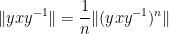
![\displaystyle f( Z ) \leq |Y_1+\dots+Y_{2n}| (\|x\| + \frac{1}{2} \| [x,y] \|),](https://s0.wp.com/latex.php?latex=%5Cdisplaystyle+f%28+Z+%29+%5Cleq+%7CY_1%2B%5Cdots%2BY_%7B2n%7D%7C+%28%5C%7Cx%5C%7C+%2B+%5Cfrac%7B1%7D%7B2%7D+%5C%7C+%5Bx%2Cy%5D+%5C%7C%29%2C&bg=ffffff&fg=000000&s=0&c=20201002)
noting that 

![\displaystyle f(0,n) \leq \sqrt{2n}( \|x\| + \frac{1}{2} \| [x,y] \|).](https://s0.wp.com/latex.php?latex=%5Cdisplaystyle+f%280%2Cn%29+%5Cleq+%5Csqrt%7B2n%7D%28+%5C%7Cx%5C%7C+%2B+%5Cfrac%7B1%7D%7B2%7D+%5C%7C+%5Bx%2Cy%5D+%5C%7C%29.&bg=ffffff&fg=000000&s=0&c=20201002)
But by (1), the left-hand side is equal to ![{n \| [x,y]\|}](https://s0.wp.com/latex.php?latex=%7Bn+%5C%7C+%5Bx%2Cy%5D%5C%7C%7D&bg=ffffff&fg=000000&s=0&c=20201002)
The above theorem reduces such seminorms to abelian groups. It is easy to see from (1) that any torsion element of such groups has zero seminorm, so we can in fact restrict to torsion-free groups, which we now write using additive notation 


This post is a continuation of the previous post, which has attracted a large number of comments. I’m recording here some calculations that arose from those comments (particularly those of Pace Nielsen, Lior Silberman, Tobias Fritz, and Apoorva Khare). Please feel free to either continue these calculations or to discuss other approaches to the problem, such as those mentioned in the remaining comments to the previous post.
Let 


and the linear growth property

for all 

or equivalently

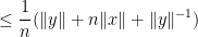
We consider inequalities of the form


for various real numbers 

we have (1) for 
Proposition 1
 .
. , then
  .
. .
.Proof: For (i) we simply observe that

For (ii), we calculate


giving the claim.
For (iii), we calculate


giving the claim.
For (iv), we calculate


giving the claim.
Here is a typical application of the above estimates. If (1) holds for 


For instance, if 

Here is a curious question posed to me by Apoorva Khare that I do not know the answer to. Let
- bi-invariant, thus
for all
; and
- linear growth in the sense that
for all
and all natural numbers
By defining the “norm” of an element 
for all 

for all
for all 
One can normalise the norm of the generators to be at most

This can then be used to upper bound the norm of other words in

A bit less trivially, from (3), (2), (1) one can bound commutators as

In a similar spirit one has

What is not clear to me is if one can keep arguing like this to continually improve the upper bounds on the norm 

I’ve just uploaded to the arXiv my paper “On the universality of the incompressible Euler equation on compact manifolds“, submitted to Discrete and Continuous Dynamical Systems. This is a variant of my recent paper on the universality of potential well dynamics, but instead of trying to embed dynamical systems into a potential well 


on a Riemannian manifold 
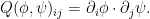
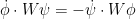
The Euler equations can be viewed as a nonlinear equation in which the nonlinearity is a quadratic function of the velocity field 
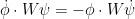
where 


for all 
For simplicity let us restrict

for some positive definite inner product 
As a consequence, any finite dimensional portion of the usual “dyadic shell models” used as simplified toy models of the Euler equation, can actually be embedded into a genuine Euler equation, albeit on a high-dimensional and curved manifold. This includes portions of the self-similar “machine” I used in a previous paper to establish finite time blowup for an averaged version of the Navier-Stokes (or Euler) equations. Unfortunately, the result in this paper does not apply to infinite-dimensional ODE, so I cannot yet establish finite time blowup for the Euler equations on a (well-chosen) manifold. It does not seem so far beyond the realm of possibility, though, that this could be done in the relatively near future. In particular, the result here suggests that one could construct something resembling a universal Turing machine within an Euler flow on a manifold, which was one ingredient I would need to engineer such a finite time blowup.
The proof of the main theorem proceeds by an “elimination of variables” strategy that was used in some of my previous papers in this area, though in this particular case the Nash embedding theorem (or variants thereof) are not required. The first step is to lessen the dependence on the metric 

Recent Comments