The structure of logarithmically averaged correlations of multiplicative functions, with applications to the Chowla and Elliott conjectures

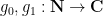
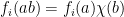
Joni Teräväinen and I have just uploaded to the arXiv our paper “The structure of logarithmically averaged correlations of multiplicative functions, with applications to the Chowla and Elliott conjectures“, submitted to Duke Mathematical Journal. This paper builds upon my previous paper in which I introduced an “entropy decrement method” to prove the two-point (logarithmically averaged) cases of the Chowla and Elliott conjectures. A bit more specifically, I showed that

whenever were sequences going to infinity, were distinct integers, and were -bounded multiplicative functions which were non-pretentious in the sense that

for all Dirichlet characters and for . Thus, for instance, one had the logarithmically averaged two-point Chowla conjecture

for fixed any non-zero , where was the Liouville function.

One would certainly like to extend these results to higher order correlations than the two-point correlations. This looks to be difficult (though perhaps not completely impossible if one allows for logarithmic averaging): in a previous paper I showed that achieving this in the context of the Liouville function would be equivalent to resolving the logarithmically averaged Sarnak conjecture, as well as establishing logarithmically averaged local Gowers uniformity of the Liouville function. However, in this paper we are able to avoid having to resolve these difficult conjectures to obtain partial results towards the (logarithmically averaged) Chowla and Elliott conjecture. For the Chowla conjecture, we can obtain all odd order correlations, in that

for all odd and all integers (which, in the odd order case, are no longer required to be distinct). (Superficially, this looks like we have resolved “half of the cases” of the logarithmically averaged Chowla conjecture; but it seems the odd order correlations are significantly easier than the even order ones. For instance, because of the Katai-Bourgain-Sarnak-Ziegler criterion, one can basically deduce the odd order cases of (2) from the even order cases (after allowing for some dilations in the argument ).

For the more general Elliott conjecture, we can show that

for any , any integers and any bounded multiplicative functions , unless the product weakly pretends to be a Dirichlet character in the sense that

This can be seen to imply (2) as a special case. Even when does pretend to be a Dirichlet character , we can still say something: if the limits

exist for each (which can be guaranteed if we pass to a suitable subsequence), then is the uniform limit of periodic functions , each of which is –isotypic in the sense that whenever are integers with coprime to the periods of and . This does not pin down the value of any single correlation , but does put significant constraints on how these correlations may vary with .

Among other things, this allows us to show that all possible length four sign patterns of the Liouville function occur with positive density, and all possible length four sign patterns occur with the conjectured logarithmic density. (In a previous paper with Matomaki and Radziwill, we obtained comparable results for length three patterns of Liouville and length two patterns of Möbius.)

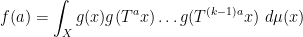
To describe the argument, let us focus for simplicity on the case of the Liouville correlations

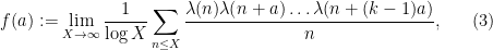
assuming for sake of discussion that all limits exist. (In the paper, we instead use the device of generalised limits, as discussed in this previous post.) The idea is to combine together two rather different ways to control this function . The first proceeds by the entropy decrement method mentioned earlier, which roughly speaking works as follows. Firstly, we pick a prime and observe that for any , which allows us to rewrite (3) as

Making the change of variables , we obtain

The difference between and is negligible in the limit (here is where we crucially rely on the log-averaging), hence

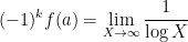
and thus by (3) we have

The entropy decrement argument can be used to show that the latter limit is small for most (roughly speaking, this is because the factors behave like independent random variables as varies, so that concentration of measure results such as Hoeffding’s inequality can apply, after using entropy inequalities to decouple somewhat these random variables from the factors). We thus obtain the approximate isotopy property

for most and .

On the other hand, by the Furstenberg correspondence principle (as discussed in these previous posts), it is possible to express as a multiple correlation

for some probability space equipped with a measure-preserving invertible map . Using results of Bergelson-Host-Kra, Leibman, and Le, this allows us to obtain a decomposition of the form

where is a nilsequence, and goes to zero in density (even along the primes, or constant multiples of the primes). The original work of Bergelson-Host-Kra required ergodicity on , which is very definitely a hypothesis that is not available here; however, the later work of Leibman removed this hypothesis, and the work of Le refined the control on so that one still has good control when restricting to primes, or constant multiples of primes.

Ignoring the small error , we can now combine (5) to conclude that

Using the equidistribution theory of nilsequences (as developed in this previous paper of Ben Green and myself), one can break up further into a periodic piece and an “irrational” or “minor arc” piece . The contribution of the minor arc piece can be shown to mostly cancel itself out after dilating by primes and averaging, thanks to Vinogradov-type bilinear sum estimates (transferred to the primes). So we end up with

which already shows (heuristically, at least) the claim that can be approximated by periodic functions which are isotopic in the sense that

But if is odd, one can use Dirichlet’s theorem on primes in arithmetic progressions to restrict to primes that are modulo the period of , and conclude now that vanishes identically, which (heuristically, at least) gives (2).

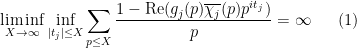
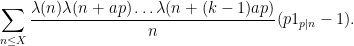
The same sort of argument works to give the more general bounds on correlations of bounded multiplicative functions. But for the specific task of proving (2), we initially used a slightly different argument that avoids using the ergodic theory machinery of Bergelson-Host-Kra, Leibman, and Le, but replaces it instead with the Gowers uniformity norm theory used to count linear equations in primes. Basically, by averaging (4) in using the “-trick”, as well as known facts about the Gowers uniformity of the von Mangoldt function, one can obtain an approximation of the form

where ranges over a large range of integers coprime to some primorial . On the other hand, by iterating (4) we have

for most semiprimes , and by again averaging over semiprimes one can obtain an approximation of the form

For odd, one can combine the two approximations to conclude that . (This argument is not given in the current paper, but we plan to detail it in a subsequent one.)

Furstenberg limits of the Liouville function

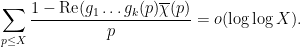
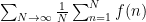
Given a function on the natural numbers taking values in , one can invoke the Furstenberg correspondence principle to locate a measure preserving system – a probability space together with a measure-preserving shift (or equivalently, a measure-preserving -action on ) – together with a measurable function (or “observable”) that has essentially the same statistics as in the sense that

for any integers . In particular, one has

 

whenever the limit on the right-hand side exists. We will refer to the system together with the designated function as a Furstenberg limit ot the sequence . These Furstenberg limits capture some, but not all, of the asymptotic behaviour of ; roughly speaking, they control the typical “local” behaviour of , involving correlations such as in the regime where are much smaller than . However, the control on error terms here is usually only qualitative at best, and one usually does not obtain non-trivial control on correlations in which the are allowed to grow at some significant rate with (e.g. like some power of ).

The correspondence principle is discussed in these previous blog posts. One way to establish the principle is by introducing a Banach limit that extends the usual limit functional on the subspace of consisting of convergent sequences while still having operator norm one. Such functionals cannot be constructed explicitly, but can be proven to exist (non-constructively and non-uniquely) using the Hahn-Banach theorem; one can also use a non-principal ultrafilter here if desired. One can then seek to construct a system and a measurable function for which one has the statistics

 

for all . One can explicitly construct such a system as follows. One can take to be the Cantor space with the product -algebra and the shift

with the function being the coordinate function at zero:

(so in particular for any ). The only thing remaining is to construct the invariant measure . In order to be consistent with (2), one must have

for any distinct integers and signs . One can check that this defines a premeasure on the Boolean algebra of defined by cylinder sets, and the existence of then follows from the Hahn-Kolmogorov extension theorem (or the closely related Kolmogorov extension theorem). One can then check that the correspondence (2) holds, and that is translation-invariant; the latter comes from the translation invariance of the (Banach-)Césaro averaging operation . A variant of this construction shows that the Furstenberg limit is unique up to equivalence if and only if all the limits appearing in (1) actually exist.

One can obtain a slightly tighter correspondence by using a smoother average than the Césaro average. For instance, one can use the logarithmic Césaro averages in place of the Césaro average , thus one replaces (2) by

Whenever the Césaro average of a bounded sequence exists, then the logarithmic Césaro average exists and is equal to the Césaro average. Thus, a Furstenberg limit constructed using logarithmic Banach-Césaro averaging still obeys (1) for all when the right-hand side limit exists, but also obeys the more general assertion

whenever the limit of the right-hand side exists.

In a recent paper of Frantizinakis, the Furstenberg limits of the Liouville function (with logarithmic averaging) were studied. Some (but not all) of the known facts and conjectures about the Liouville function can be interpreted in the Furstenberg limit. For instance, in a recent breakthrough result of Matomaki and Radziwill (discussed previously here), it was shown that the Liouville function exhibited cancellation on short intervals in the sense that

In terms of Furstenberg limits of the Liouville function, this assertion is equivalent to the assertion that

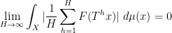
for all Furstenberg limits of Liouville (including those without logarithmic averaging). Invoking the mean ergodic theorem (discussed in this previous post), this assertion is in turn equivalent to the observable that corresponds to the Liouville function being orthogonal to the invariant factor of ; equivalently, the first Gowers-Host-Kra seminorm of (as defined for instance in this previous post) vanishes. The Chowla conjecture, which asserts that

for all distinct integers , is equivalent to the assertion that all the Furstenberg limits of Liouville are equivalent to the Bernoulli system ( with the product measure arising from the uniform distribution on , with the shift and observable as before). Similarly, the logarithmically averaged Chowla conjecture

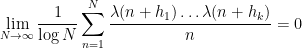
is equivalent to the assertion that all the Furstenberg limits of Liouville with logarithmic averaging are equivalent to the Bernoulli system. Recently, I was able to prove the two-point version

 

of the logarithmically averaged Chowla conjecture, for any non-zero integer ; this is equivalent to the perfect strong mixing property

for any Furstenberg limit of Liouville with logarithmic averaging, and any .

The situation is more delicate with regards to the Sarnak conjecture, which is equivalent to the assertion that

for any zero-entropy sequence (see this previous blog post for more discussion). Morally speaking, this conjecture should be equivalent to the assertion that any Furstenberg limit of Liouville is disjoint from any zero entropy system, but I was not able to formally establish an implication in either direction due to some technical issues regarding the fact that the Furstenberg limit does not directly control long-range correlations, only short-range ones. (There are however ergodic theoretic interpretations of the Sarnak conjecture that involve the notion of generic points; see this paper of El Abdalaoui, Lemancyk, and de la Rue.) But the situation is currently better with the logarithmically averaged Sarnak conjecture

as I was able to show that this conjecture was equivalent to the logarithmically averaged Chowla conjecture, and hence to all Furstenberg limits of Liouville with logarithmic averaging being Bernoulli; I also showed the conjecture was equivalent to local Gowers uniformity of the Liouville function, which is in turn equivalent to the function having all Gowers-Host-Kra seminorms vanishing in every Furstenberg limit with logarithmic averaging. In this recent paper of Frantzikinakis, this analysis was taken further, showing that the logarithmically averaged Chowla and Sarnak conjectures were in fact equivalent to the much milder seeming assertion that all Furstenberg limits with logarithmic averaging were ergodic.

Actually, the logarithmically averaged Furstenberg limits have more structure than just a -action on a measure preserving system with a single observable . Let denote the semigroup of affine maps on the integers with and positive. Also, let denote the profinite integers (the inverse limit of the cyclic groups ). Observe that acts on by taking the inverse limit of the obvious actions of on .

Proposition 1 (Enriched logarithmically averaged Furstenberg limit of Liouville) Let be a Banach limit. Then there exists a probability space with an action of the affine semigroup , as well as measurable functions and , with the following properties:

• (i) (Affine Furstenberg limit) For any , and any congruence class , one has

  

  

• (ii) (Equivariance of ) For any , one has

  

  for -almost every .

• (iii) (Multiplicativity at fixed primes) For any prime , one has

  

  for -almost every , where is the dilation map .

• (iv) (Measure pushforward) If is of the form and is the set , then the pushforward of by is equal to , that is to say one has

  

  for every measurable .

Note that can be viewed as the subgroup of consisting of the translations . If one only keeps the -portion of the action and forgets the rest (as well as the function ) then the action becomes measure-preserving, and we recover an ordinary Furstenberg limit with logarithmic averaging. However, the additional structure here can be quite useful; for instance, one can transfer the proof of (3) to this setting, which we sketch below the fold, after proving the proposition.

The observable , roughly speaking, means that points in the Furstenberg limit constructed by this proposition are still “virtual integers” in the sense that one can meaningfully compute the residue class of modulo any natural number modulus , by first applying and then reducing mod . The action of means that one can also meaningfully multiply by any natural number, and translate it by any integer. As with other applications of the correspondence principle, the main advantage of moving to this more “virtual” setting is that one now acquires a probability measure , so that the tools of ergodic theory can be readily applied.

Ultraproducts as a Bridge Between Discrete and Continuous Analysis

(This is an extended blog post version of my talk “Ultraproducts as a Bridge Between Discrete and Continuous Analysis” that I gave at the Simons institute for the theory of computing at the workshop “Neo-Classical methods in discrete analysis“. Some of the material here is drawn from previous blog posts, notably “Ultraproducts as a bridge between hard analysis and soft analysis” and “Ultralimit analysis and quantitative algebraic geometry“‘. The text here has substantially more details than the talk; one may wish to skip all of the proofs given here to obtain a closer approximation to the original talk.)

Discrete analysis, of course, is primarily interested in the study of discrete (or “finitary”) mathematical objects: integers, rational numbers (which can be viewed as ratios of integers), finite sets, finite graphs, finite or discrete metric spaces, and so forth. However, many powerful tools in mathematics (e.g. ergodic theory, measure theory, topological group theory, algebraic geometry, spectral theory, etc.) work best when applied to continuous (or “infinitary”) mathematical objects: real or complex numbers, manifolds, algebraic varieties, continuous topological or metric spaces, etc. In order to apply results and ideas from continuous mathematics to discrete settings, there are basically two approaches. One is to directly discretise the arguments used in continuous mathematics, which often requires one to keep careful track of all the bounds on various quantities of interest, particularly with regard to various error terms arising from discretisation which would otherwise have been negligible in the continuous setting. The other is to construct continuous objects as limits of sequences of discrete objects of interest, so that results from continuous mathematics may be applied (often as a “black box”) to the continuous limit, which then can be used to deduce consequences for the original discrete objects which are quantitative (though often ineffectively so). The latter approach is the focus of this current talk.

The following table gives some examples of a discrete theory and its continuous counterpart, together with a limiting procedure that might be used to pass from the former to the latter:

(Discrete)	(Continuous)	(Limit method)
Ramsey theory	Topological dynamics	Compactness
Density Ramsey theory	Ergodic theory	Furstenberg correspondence principle
Graph/hypergraph regularity	Measure theory	Graph limits
Polynomial regularity	Linear algebra	Ultralimits
Structural decompositions	Hilbert space geometry	Ultralimits
Fourier analysis	Spectral theory	Direct and inverse limits
Quantitative algebraic geometry	Algebraic geometry	Schemes
Discrete metric spaces	Continuous metric spaces	Gromov-Hausdorff limits
Approximate group theory	Topological group theory	Model theory

As the above table illustrates, there are a variety of different ways to form a limiting continuous object. Roughly speaking, one can divide limits into three categories:

• Topological and metric limits. These notions of limits are commonly used by analysts. Here, one starts with a sequence (or perhaps a net) of objects in a common space , which one then endows with the structure of a topological space or a metric space, by defining a notion of distance between two points of the space, or a notion of open neighbourhoods or open sets in the space. Provided that the sequence or net is convergent, this produces a limit object , which remains in the same space, and is “close” to many of the original objects with respect to the given metric or topology.
• Categorical limits. These notions of limits are commonly used by algebraists. Here, one starts with a sequence (or more generally, a diagram) of objects in a category , which are connected to each other by various morphisms. If the ambient category is well-behaved, one can then form the direct limit or the inverse limit of these objects, which is another object in the same category , and is connected to the original objects by various morphisms.
• Logical limits. These notions of limits are commonly used by model theorists. Here, one starts with a sequence of objects or of spaces , each of which is (a component of) a model for given (first-order) mathematical language (e.g. if one is working in the language of groups, might be groups and might be elements of these groups). By using devices such as the ultraproduct construction, or the compactness theorem in logic, one can then create a new object or a new space , which is still a model of the same language (e.g. if the spaces were all groups, then the limiting space will also be a group), and is “close” to the original objects or spaces in the sense that any assertion (in the given language) that is true for the limiting object or space, will also be true for many of the original objects or spaces, and conversely. (For instance, if is an abelian group, then the will also be abelian groups for many .)

The purpose of this talk is to highlight the third type of limit, and specifically the ultraproduct construction, as being a “universal” limiting procedure that can be used to replace most of the limits previously mentioned. Unlike the topological or metric limits, one does not need the original objects to all lie in a common space in order to form an ultralimit ; they are permitted to lie in different spaces ; this is more natural in many discrete contexts, e.g. when considering graphs on vertices in the limit when goes to infinity. Also, no convergence properties on the are required in order for the ultralimit to exist. Similarly, ultraproduct limits differ from categorical limits in that no morphisms between the various spaces involved are required in order to construct the ultraproduct.

With so few requirements on the objects or spaces , the ultraproduct construction is necessarily a very “soft” one. Nevertheless, the construction has two very useful properties which make it particularly useful for the purpose of extracting good continuous limit objects out of a sequence of discrete objects. First of all, there is Łos’s theorem, which roughly speaking asserts that any first-order sentence which is asymptotically obeyed by the , will be exactly obeyed by the limit object ; in particular, one can often take a discrete sequence of “partial counterexamples” to some assertion, and produce a continuous “complete counterexample” that same assertion via an ultraproduct construction; taking the contrapositives, one can often then establish a rigorous equivalence between a quantitative discrete statement and its qualitative continuous counterpart. Secondly, there is the countable saturation property that ultraproducts automatically enjoy, which is a property closely analogous to that of compactness in topological spaces, and can often be used to ensure that the continuous objects produced by ultraproduct methods are “complete” or “compact” in various senses, which is particularly useful in being able to upgrade qualitative (or “pointwise”) bounds to quantitative (or “uniform”) bounds, more or less “for free”, thus reducing significantly the burden of “epsilon management” (although the price one pays for this is that one needs to pay attention to which mathematical objects of study are “standard” and which are “nonstandard”). To achieve this compactness or completeness, one sometimes has to restrict to the “bounded” portion of the ultraproduct, and it is often also convenient to quotient out the “infinitesimal” portion in order to complement these compactness properties with a matching “Hausdorff” property, thus creating familiar examples of continuous spaces, such as locally compact Hausdorff spaces.

Ultraproducts are not the only logical limit in the model theorist’s toolbox, but they are one of the simplest to set up and use, and already suffice for many of the applications of logical limits outside of model theory. In this post, I will set out the basic theory of these ultraproducts, and illustrate how they can be used to pass between discrete and continuous theories in each of the examples listed in the above table.

Apart from the initial “one-time cost” of setting up the ultraproduct machinery, the main loss one incurs when using ultraproduct methods is that it becomes very difficult to extract explicit quantitative bounds from results that are proven by transferring qualitative continuous results to the discrete setting via ultraproducts. However, in many cases (particularly those involving regularity-type lemmas) the bounds are already of tower-exponential type or worse, and there is arguably not much to be lost by abandoning the explicit quantitative bounds altogether.

A multi-dimensional Szemer\’edi theorem for the primes via a correspondence principle

Tamar Ziegler and I have just uploaded to the arXiv our joint paper “A multi-dimensional Szemerédi theorem for the primes via a correspondence principle“. This paper is related to an earlier result of Ben Green and mine in which we established that the primes contain arbitrarily long arithmetic progressions. Actually, in that paper we proved a more general result:

Theorem 1 (Szemerédi’s theorem in the primes) Let be a subset of the primes of positive relative density, thus . Then contains arbitrarily long arithmetic progressions.

This result was based in part on an earlier paper of Green that handled the case of progressions of length three. With the primes replaced by the integers, this is of course the famous theorem of Szemerédi.

Szemerédi’s theorem has now been generalised in many different directions. One of these is the multidimensional Szemerédi theorem of Furstenberg and Katznelson, who used ergodic-theoretic techniques to show that any dense subset of necessarily contained infinitely many constellations of any prescribed shape. Our main result is to relativise that theorem to the primes as well:

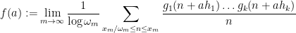
Theorem 2 (Multidimensional Szemerédi theorem in the primes) Let , and let be a subset of the Cartesian power of the primes of positive relative density, thus

Then for any , contains infinitely many “constellations” of the form with and a positive integer.

In the case when is itself a Cartesian product of one-dimensional sets (in particular, if is all of ), this result already follows from Theorem 1, but there does not seem to be a similarly easy argument to deduce the general case of Theorem 2 from previous results. Simultaneously with this paper, an independent proof of Theorem 2 using a somewhat different method has been established by Cook, Maygar, and Titichetrakun.

The result is reminiscent of an earlier result of mine on finding constellations in the Gaussian primes (or dense subsets thereof). That paper followed closely the arguments of my original paper with Ben Green, namely it first enclosed (a W-tricked version of) the primes or Gaussian primes (in a sieve theoretic-sense) by a slightly larger set (or more precisely, a weight function ) of almost primes or almost Gaussian primes, which one could then verify (using methods closely related to the sieve-theoretic methods in the ongoing Polymath8 project) to obey certain pseudorandomness conditions, known as the linear forms condition and the correlation condition. Very roughly speaking, these conditions assert statements of the following form: if is a randomly selected integer, then the events of simultaneously being an almost prime (or almost Gaussian prime) are approximately independent for most choices of . Once these conditions are satisfied, one can then run a transference argument (initially based on ergodic-theory methods, but nowadays there are simpler transference results based on the Hahn-Banach theorem, due to Gowers and Reingold-Trevisan-Tulsiani-Vadhan) to obtain relative Szemerédi-type theorems from their absolute counterparts.

However, when one tries to adapt these arguments to sets such as , a new difficulty occurs: the natural analogue of the almost primes would be the Cartesian square of the almost primes – pairs whose entries are both almost primes. (Actually, for technical reasons, one does not work directly with a set of almost primes, but would instead work with a weight function such as that is concentrated on a set such as , but let me ignore this distinction for now.) However, this set does not enjoy as many pseudorandomness conditions as one would need for a direct application of the transference strategy to work. More specifically, given any fixed , and random , the four events

do not behave independently (as they would if were replaced for instance by the Gaussian almost primes), because any three of these events imply the fourth. This blocks the transference strategy for constellations which contain some right-angles to them (e.g. constellations of the form ) as such constellations soon turn into rectangles such as the one above after applying Cauchy-Schwarz a few times. (But a few years ago, Cook and Magyar showed that if one restricted attention to constellations which were in general position in the sense that any coordinate hyperplane contained at most one element in the constellation, then this obstruction does not occur and one can establish Theorem 2 in this case through the transference argument.) It’s worth noting that very recently, Conlon, Fox, and Zhao have succeeded in removing of the pseudorandomness conditions (namely the correlation condition) from the transference principle, leaving only the linear forms condition as the remaining pseudorandomness condition to be verified, but unfortunately this does not completely solve the above problem because the linear forms condition also fails for (or for weights concentrated on ) when applied to rectangular patterns.

There are now two ways known to get around this problem and establish Theorem 2 in full generality. The approach of Cook, Magyar, and Titichetrakun proceeds by starting with one of the known proofs of the multidimensional Szemerédi theorem – namely, the proof that proceeds through hypergraph regularity and hypergraph removal – and attach pseudorandom weights directly within the proof itself, rather than trying to add the weights to the result of that proof through a transference argument. (A key technical issue is that weights have to be added to all the levels of the hypergraph – not just the vertices and top-order edges – in order to circumvent the failure of naive pseudorandomness.) As one has to modify the entire proof of the multidimensional Szemerédi theorem, rather than use that theorem as a black box, the Cook-Magyar-Titichetrakun argument is lengthier than ours; on the other hand, it is more general and does not rely on some difficult theorems about primes that are used in our paper.

In our approach, we continue to use the multidimensional Szemerédi theorem (or more precisely, the equivalent theorem of Furstenberg and Katznelson concerning multiple recurrence for commuting shifts) as a black box. The difference is that instead of using a transference principle to connect the relative multidimensional Szemerédi theorem we need to the multiple recurrence theorem, we instead proceed by a version of the Furstenberg correspondence principle, similar to the one that connects the absolute multidimensional Szemerédi theorem to the multiple recurrence theorem. I had discovered this approach many years ago in an unpublished note, but had abandoned it because it required an infinite number of linear forms conditions (in contrast to the transference technique, which only needed a finite number of linear forms conditions and (until the recent work of Conlon-Fox-Zhao) a correlation condition). The reason for this infinite number of conditions is that the correspondence principle has to build a probability measure on an entire -algebra; for this, it is not enough to specify the measure of a single set such as , but one also has to specify the measure of “cylinder sets” such as where could be arbitrarily large. The larger gets, the more linear forms conditions one needs to keep the correspondence under control.

With the sieve weights we were using at the time, standard sieve theory methods could indeed provide a finite number of linear forms conditions, but not an infinite number, so my idea was abandoned. However, with my later work with Green and Ziegler on linear equations in primes (and related work on the Mobius-nilsequences conjecture and the inverse conjecture on the Gowers norm), Tamar and I realised that the primes themselves obey an infinite number of linear forms conditions, so one can basically use the primes (or a proxy for the primes, such as the von Mangoldt function ) as the enveloping sieve weight, rather than a classical sieve. Thus my old idea of using the Furstenberg correspondence principle to transfer Szemerédi-type theorems to the primes could actually be realised. In the one-dimensional case, this simply produces a much more complicated proof of Theorem 1 than the existing one; but it turns out that the argument works as well in higher dimensions and yields Theorem 2 relatively painlessly, except for the fact that it needs the results on linear equations in primes, the known proofs of which are extremely lengthy (and also require some of the transference machinery mentioned earlier). The problem of correlations in rectangles is avoided in the correspondence principle approach because one can compensate for such correlations by performing a suitable weighted limit to compute the measure of cylinder sets, with each requiring a different weighted correction. (This may be related to the Cook-Magyar-Titichetrakun strategy of weighting all of the facets of the hypergraph in order to recover pseudorandomness, although our contexts are rather different.)

An informal version of the Furstenberg correspondence principle

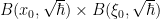
One of the basic objects of study in combinatorics are finite strings or infinite strings of symbols from some given alphabet , which could be either finite or infinite (but which we shall usually take to be compact). For instance, a set of natural numbers can be identified with the infinite string of s and s formed by the indicator of , e.g. the even numbers can be identified with the string from the alphabet , the multiples of three can be identified with the string , and so forth. One can also consider doubly infinite strings , which among other things can be used to describe arbitrary subsets of integers.

On the other hand, the basic object of study in dynamics (and in related fields, such as ergodic theory) is that of a dynamical system , that is to say a space together with a shift map (which is often assumed to be invertible, although one can certainly study non-invertible dynamical systems as well). One often adds additional structure to this dynamical system, such as topological structure (giving rise topological dynamics), measure-theoretic structure (giving rise to ergodic theory), complex structure (giving rise to complex dynamics), and so forth. A dynamical system gives rise to an action of the natural numbers on the space by using the iterates of for ; if is invertible, we can extend this action to an action of the integers on the same space. One can certainly also consider dynamical systems whose underlying group (or semi-group) is something other than or (e.g. one can consider continuous dynamical systems in which the evolution group is ), but we will restrict attention to the classical situation of or actions here.

There is a fundamental correspondence principle connecting the study of strings (or subsets of natural numbers or integers) with the study of dynamical systems. In one direction, given a dynamical system , an observable taking values in some alphabet , and some initial datum , we can first form the forward orbit of , and then observe this orbit using to obtain an infinite string . If the shift in this system is invertible, one can extend this infinite string into a doubly infinite string . Thus we see that every quadruplet consisting of a dynamical system , an observable , and an initial datum creates an infinite string.

Example 1 If is the three-element set with the shift map , is the observable that takes the value at the residue class and zero at the other two classes, and one starts with the initial datum , then the observed string becomes the indicator of the multiples of three.

In the converse direction, every infinite string in some alphabet arises (in a decidedly non-unique fashion) from a quadruple in the above fashion. This can be easily seen by the following “universal” construction: take to be the set of infinite strings in the alphabet , let be the shift map

let be the observable

and let be the initial point

Then one easily sees that the observed string is nothing more than the original string . Note also that this construction can easily be adapted to doubly infinite strings by using instead of , at which point the shift map now becomes invertible. An important variant of this construction also attaches an invariant probability measure to that is associated to the limiting density of various sets associated to the string , and leads to the Furstenberg correspondence principle, discussed for instance in these previous blog posts. Such principles allow one to rigorously pass back and forth between the combinatorics of strings and the dynamics of systems; for instance, Furstenberg famously used his correspondence principle to demonstrate the equivalence of Szemerédi’s theorem on arithmetic progressions with what is now known as the Furstenberg multiple recurrence theorem in ergodic theory.

In the case when the alphabet is the binary alphabet , and (for technical reasons related to the infamous non-injectivity of the decimal representation system) the string does not end with an infinite string of s, then one can reformulate the above universal construction by taking to be the interval , to be the doubling map , to be the observable that takes the value on and on (that is, is the first binary digit of ), and is the real number (that is, in binary).

The above universal construction is very easy to describe, and is well suited for “generic” strings that have no further obvious structure to them, but it often leads to dynamical systems that are much larger and more complicated than is actually needed to produce the desired string , and also often obscures some of the key dynamical features associated to that sequence. For instance, to generate the indicator of the multiples of three that were mentioned previously, the above universal construction requires an uncountable space and a dynamics which does not obviously reflect the key features of the sequence such as its periodicity. (Using the unit interval model, the dynamics arise from the orbit of under the doubling map, which is a rather artificial way to describe the indicator function of the multiples of three.)

A related aesthetic objection to the universal construction is that of the four components of the quadruplet used to generate the sequence , three of the components are completely universal (in that they do not depend at all on the sequence ), leaving only the initial datum to carry all the distinctive features of the original sequence. While there is nothing wrong with this mathematically, from a conceptual point of view it would make sense to make all four components of the quadruplet to be adapted to the sequence, in order to take advantage of the accumulated intuition about various special dynamical systems (and special observables), not just special initial data.

One step in this direction can be made by restricting to the orbit of the initial datum (actually for technical reasons it is better to restrict to the topological closure of this orbit, in order to keep compact). For instance, starting with the sequence , the orbit now consists of just three points , , , bringing the system more in line with the example in Example 1. Technically, this is the “optimal” representation of the sequence by a quadruplet , because any other such representation is a factor of this representation (in the sense that there is a unique map with , , and ). However, from a conceptual point of view this representation is still somewhat unsatisfactory, given that the elements of the system are interpreted as infinite strings rather than elements of a more geometrically or algebraically rich object (e.g. points in a circle, torus, or other homogeneous space).

For general sequences , locating relevant geometric or algebraic structure in a dynamical system generating that sequence is an important but very difficult task (see e.g. this paper of Host and Kra, which is more or less devoted to precisely this task in the context of working out what component of a dynamical system controls the multiple recurrence behaviour of that system). However, for specific examples of sequences , one can use an informal procedure of educated guesswork in order to produce a more natural-looking quadruple that generates that sequence. This is not a particularly difficult or deep operation, but I found it very helpful in internalising the intuition behind the correspondence principle. Being non-rigorous, this procedure does not seem to be emphasised in most presentations of the correspondence principle, so I thought I would describe it here.

Lars Hormander

Lars Hörmander, who made fundamental contributions to all areas of partial differential equations, but particularly in developing the analysis of variable-coefficient linear PDE, died last Sunday, aged 81.

I unfortunately never met Hörmander personally, but of course I encountered his work all the time while working in PDE. One of his major contributions to the subject was to systematically develop the calculus of Fourier integral operators (FIOs), which are a substantial generalisation of pseudodifferential operators and which can be used to (approximately) solve linear partial differential equations, or to transform such equations into a more convenient form. Roughly speaking, Fourier integral operators are to linear PDE as canonical transformations are to Hamiltonian mechanics (and one can in fact view FIOs as a quantisation of a canonical transformation). They are a large class of transformations, for instance the Fourier transform, pseudodifferential operators, and smooth changes of the spatial variable are all examples of FIOs, and (as long as certain singular situations are avoided) the composition of two FIOs is again an FIO.

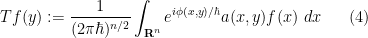
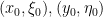
The full theory of FIOs is quite extensive, occupying the entire final volume of Hormander’s famous four-volume series “The Analysis of Linear Partial Differential Operators”. I am certainly not going to try to attempt to summarise it here, but I thought I would try to motivate how these operators arise when trying to transform functions. For simplicity we will work with functions on a Euclidean domain (although FIOs can certainly be defined on more general smooth manifolds, and there is an extension of the theory that also works on manifolds with boundary). As this will be a heuristic discussion, we will ignore all the (technical, but important) issues of smoothness or convergence with regards to the functions, integrals and limits that appear below, and be rather vague with terms such as “decaying” or “concentrated”.

A function can be viewed from many different perspectives (reflecting the variety of bases, or approximate bases, that the Hilbert space offers). Most directly, we have the physical space perspective, viewing as a function of the physical variable . In many cases, this function will be concentrated in some subregion of physical space. For instance, a gaussian wave packet

where , and are parameters, would be physically concentrated in the ball . Then we have the frequency space (or momentum space) perspective, viewing now as a function of the frequency variable . For this discussion, it will be convenient to normalise the Fourier transform using a small constant (which has the physical interpretation of Planck’s constant if one is doing quantum mechanics), thus

For instance, for the gaussian wave packet (1), one has

and so we see that is concentrated in frequency space in the ball .

However, there is a third (but less rigorous) way to view a function in , which is the phase space perspective in which one tries to view as distributed simultaneously in physical space and in frequency space, thus being something like a measure on the phase space . Thus, for instance, the function (1) should heuristically be concentrated on the region in phase space. Unfortunately, due to the uncertainty principle, there is no completely satisfactory way to canonically and rigorously define what the “phase space portrait” of a function should be. (For instance, the Wigner transform of can be viewed as an attempt to describe the distribution of the energy of in phase space, except that this transform can take negative or even complex values; see Folland’s book for further discussion.) Still, it is a very useful heuristic to think of functions has having a phase space portrait, which is something like a non-negative measure on phase space that captures the distribution of functions in both space and frequency, albeit with some “quantum fuzziness” that shows up whenever one tries to inspect this measure at scales of physical space and frequency space that together violate the uncertainty principle. (The score of a piece of music is a good everyday example of a phase space portrait of a function, in this case a sound wave; here, the physical space is the time axis (the horizontal dimension of the score) and the frequency space is the vertical dimension. Here, the time and frequency scales involved are well above the uncertainty principle limit (a typical note lasts many hundreds of cycles, whereas the uncertainty principle kicks in at cycles) and so there is no obstruction here to musical notation being unambiguous.) Furthermore, if one takes certain asymptotic limits, one can recover a precise notion of a phase space portrait; for instance if one takes the semiclassical limit then, under certain circumstances, the phase space portrait converges to a well-defined classical probability measure on phase space; closely related to this is the high frequency limit of a fixed function, which among other things defines the wave front set of that function, which can be viewed as another asymptotic realisation of the phase space portrait concept.

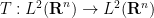
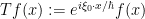
If functions in can be viewed as a sort of distribution in phase space, then linear operators should be viewed as various transformations on such distributions on phase space. For instance, a pseudodifferential operator should correspond (as a zeroth approximation) to multiplying a phase space distribution by the symbol of that operator, as discussed in this previous blog post. Note that such operators only change the amplitude of the phase space distribution, but not the support of that distribution.

Now we turn to operators that alter the support of a phase space distribution, rather than the amplitude; we will focus on unitary operators to emphasise the amplitude preservation aspect. These will eventually be key examples of Fourier integral operators. A physical translation 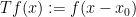should correspond to pushing forward the distribution by the transformation , as can be seen by comparing the physical and frequency space supports of with that of . Similarly, a frequency modulation should correspond to the transformation ; a linear change of variables , where is an invertible linear transformation, should correspond to ; and finally, the Fourier transform should correspond to the transformation .

Based on these examples, one may hope that given any diffeomorphism of phase space, one could associate some sort of unitary (or approximately unitary) operator , which (heuristically, at least) pushes the phase space portrait of a function forward by . However, there is an obstruction to doing so, which can be explained as follows. If pushes phase space portraits by , and pseudodifferential operators multiply phase space portraits by , then this suggests the intertwining relationship

and thus is approximately conjugate to :

The formalisation of this fact in the theory of Fourier integral operators is known as Egorov’s theorem, due to Yu Egorov (and not to be confused with the more widely known theorem of Dmitri Egorov in measure theory).

Applying commutators, we conclude the approximate conjugacy relationship

Now, the pseudodifferential calculus (as discussed in this previous post) tells us (heuristically, at least) that

and

where is the Poisson bracket. Comparing this with (2), we are then led to the compatibility condition

thus needs to preserve (approximately, at least) the Poisson bracket, or equivalently needs to be a symplectomorphism (again, approximately at least).

Now suppose that is a symplectomorphism. This is morally equivalent to the graph being a Lagrangian submanifold of (where we give the second copy of phase space the negative of the usual symplectic form , thus yielding as the full symplectic form on ; this is another instantiation of the closed graph theorem, as mentioned in this previous post. This graph is known as the canonical relation for the (putative) FIO that is associated to . To understand what it means for this graph to be Lagrangian, we coordinatise as suppose temporarily that this graph was (locally, at least) a smooth graph in the and variables, thus

for some smooth functions . A brief computation shows that the Lagrangian property of is then equivalent to the compatibility conditions

for , where denote the components of . Some Fourier analysis (or Hodge theory) lets us solve these equations as

for some smooth potential function . Thus, we have parameterised our graph as

so that maps to .

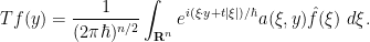
A reasonable candidate for an operator associated to and in this fashion is the oscillatory integral operator

for some smooth amplitude function (note that the Fourier transform is the special case when and , which helps explain the genesis of the term “Fourier integral operator”). Indeed, if one computes an inner product for gaussian wave packets of the form (1) and localised in phase space near respectively, then a Taylor expansion of around , followed by a stationary phase computation, shows (again heuristically, and assuming is suitably non-degenerate) that has (3) as its canonical relation. (Furthermore, a refinement of this stationary phase calculation suggests that if is normalised to be the half-density , then should be approximately unitary.) As such, we view (4) as an example of a Fourier integral operator (assuming various smoothness and non-degeneracy hypotheses on the phase and amplitude which we do not detail here).

Of course, it may be the case that is not a graph in the coordinates (for instance, the key examples of translation, modulation, and dilation are not of this form), but then it is often a graph in some other pair of coordinates, such as . In that case one can compose the oscillatory integral construction given above with a Fourier transform, giving another class of FIOs of the form

This class of FIOs covers many important cases; for instance, the translation, modulation, and dilation operators considered earlier can be written in this form after some Fourier analysis. Another typical example is the half-wave propagator for some time , which can be written in the form

This corresponds to the phase space transformation , which can be viewed as the classical propagator associated to the “quantum” propagator . More generally, propagators for linear Hamiltonian partial differential equations can often be expressed (at least approximately) by Fourier integral operators corresponding to the propagator of the associated classical Hamiltonian flow associated to the symbol of the Hamiltonian operator ; this leads to an important mathematical formalisation of the correspondence principle between quantum mechanics and classical mechanics, that is one of the foundations of microlocal analysis and which was extensively developed in Hörmander’s work. (More recently, numerically stable versions of this theory have been developed to allow for rapid and accurate numerical solutions to various linear PDE, for instance through Emmanuel Candés’ theory of curvelets, so the theory that Hörmander built now has some quite significant practical applications in areas such as geology.)

In some cases, the canonical relation may have some singularities (such as fold singularities) which prevent it from being written as graphs in the previous senses, but the theory for defining FIOs even in these cases, and in developing their calculus, is now well established, in large part due to the foundational work of Hörmander.

Nonstandard analysis as a completion of standard analysis

Many structures in mathematics are incomplete in one or more ways. For instance, the field of rationals or the reals are algebraically incomplete, because there are some non-trivial algebraic equations (such as in the case of the rationals, or in the case of the reals) which could potentially have solutions (because they do not imply a necessarily false statement, such as , just using the laws of algebra), but do not actually have solutions in the specified field.

Similarly, the rationals , when viewed now as a metric space rather than as a field, are also metrically incomplete, beause there exist sequences in the rationals (e.g. the decimal approximations of the irrational number ) which could potentially converge to a limit (because they form a Cauchy sequence), but do not actually converge in the specified metric space.

A third type of incompleteness is that of logical incompleteness, which applies now to formal theories rather than to fields or metric spaces. For instance, Zermelo-Frankel-Choice (ZFC) set theory is logically incomplete, because there exist statements (such as the consistency of ZFC) which could potentially be provable by the theory (because it does not lead to a contradiction, or at least so we believe, just from the axioms and deductive rules of the theory), but is not actually provable in this theory.

A fourth type of incompleteness, which is slightly less well known than the above three, is what I will call elementary incompleteness (and which model theorists call the failure of the countable saturation property). It applies to any structure that is describable by a first-order language, such as a field, a metric space, or a universe of sets. For instance, in the language of ordered real fields, the real line is elementarily incomplete, because there exists a sequence of statements (such as the statements for natural numbers ) in this language which are potentially simultaneously satisfiable (in the sense that any finite number of these statements can be satisfied by some real number ) but are not actually simultaneously satisfiable in this theory.

In each of these cases, though, it is possible to start with an incomplete structure and complete it to a much larger structure to eliminate the incompleteness. For instance, starting with an arbitrary field , one can take its algebraic completion (or algebraic closure) ; for instance, can be viewed as the algebraic completion of . This field is usually significantly larger than the original field , but contains as a subfield, and every element of can be described as the solution to some polynomial equation with coefficients in . Furthermore, is now algebraically complete (or algebraically closed): every polynomial equation in which is potentially satisfiable (in the sense that it does not lead to a contradiction such as from the laws of algebra), is actually satisfiable in .

Similarly, starting with an arbitrary metric space , one can take its metric completion ; for instance, can be viewed as the metric completion of . Again, the completion is usually much larger than the original metric space , but contains as a subspace, and every element of can be described as the limit of some Cauchy sequence in . Furthermore, is now a complete metric space: every sequence in which is potentially convergent (in the sense of being a Cauchy sequence), is now actually convegent in .

In a similar vein, we have the Gödel completeness theorem, which implies (among other things) that for any consistent first-order theory for a first-order language , there exists at least one completion of that theory , which is a consistent theory in which every sentence in which is potentially true in (because it does not lead to a contradiction in ) is actually true in . Indeed, the completeness theorem provides at least one model (or structure) of the consistent theory , and then the completion can be formed by interpreting every sentence in using to determine its truth value. Note, in contrast to the previous two examples, that the completion is usually not unique in any way; a theory can have multiple inequivalent models , giving rise to distinct completions of the same theory.

Finally, if one starts with an arbitrary structure , one can form an elementary completion of it, which is a significantly larger structure which contains as a substructure, and such that every element of is an elementary limit of a sequence of elements in (I will define this term shortly). Furthermore, is elementarily complete; any sequence of statements that are potentially simultaneously satisfiable in (in the sense that any finite number of statements in this collection are simultaneously satisfiable), will actually be simultaneously satisfiable. As we shall see, one can form such an elementary completion by taking an ultrapower of the original structure . If is the standard universe of all the standard objects one considers in mathematics, then its elementary completion is known as the nonstandard universe, and is the setting for nonstandard analysis.

As mentioned earlier, completion tends to make a space much larger and more complicated. If one algebraically completes a finite field, for instance, one necessarily obtains an infinite field as a consequence. If one metrically completes a countable metric space with no isolated points, such as , then one necessarily obtains an uncountable metric space (thanks to the Baire category theorem). If one takes a logical completion of a consistent first-order theory that can model true arithmetic, then this completion is no longer describable by a recursively enumerable schema of axioms, thanks to Gödel’s incompleteness theorem. And if one takes the elementary completion of a countable structure, such as the integers , then the resulting completion will necessarily be uncountable.

However, there are substantial benefits to working in the completed structure which can make it well worth the massive increase in size. For instance, by working in the algebraic completion of a field, one gains access to the full power of algebraic geometry. By working in the metric completion of a metric space, one gains access to powerful tools of real analysis, such as the Baire category theorem, the Heine-Borel theorem, and (in the case of Euclidean completions) the Bolzano-Weierstrass theorem. By working in a logically and elementarily completed theory (aka a saturated model) of a first-order theory, one gains access to the branch of model theory known as definability theory, which allows one to analyse the structure of definable sets in much the same way that algebraic geometry allows one to analyse the structure of algebraic sets. Finally, when working in an elementary completion of a structure, one gains a sequential compactness property, analogous to the Bolzano-Weierstrass theorem, which can be interpreted as the foundation for much of nonstandard analysis, as well as providing a unifying framework to describe various correspondence principles between finitary and infinitary mathematics.

In this post, I wish to expand upon these above points with regard to elementary completion, and to present nonstandard analysis as a completion of standard analysis in much the same way as, say, complex algebra is a completion of real algebra, or real metric geometry is a completion of rational metric geometry.

Szemeredi’s regularity lemma via the correspondence principle

In a previous post, we discussed the Szemerédi regularity lemma, and how a given graph could be regularised by partitioning the vertex set into random neighbourhoods. More precisely, we gave a proof of

Lemma 1 (Regularity lemma via random neighbourhoods) Let . Then there exists integers with the following property: whenever be a graph on finitely many vertices, if one selects one of the integers at random from , then selects vertices uniformly from at random, then the vertex cells (some of which can be empty) generated by the vertex neighbourhoods for , will obey the regularity property

with probability at least , where the sum is over all pairs for which is not -regular between and . [Recall that a pair is -regular for if one has

for any and with , where is the density of edges between and .]

The proof was a combinatorial one, based on the standard energy increment argument.

In this post I would like to discuss an alternate approach to the regularity lemma, which is an infinitary approach passing through a graph-theoretic version of the Furstenberg correspondence principle (mentioned briefly in this earlier post of mine). While this approach superficially looks quite different from the combinatorial approach, it in fact uses many of the same ingredients, most notably a reliance on random neighbourhoods to regularise the graph. This approach was introduced by myself back in 2006, and used by Austin and by Austin and myself to establish some property testing results for hypergraphs; more recently, a closely related infinitary hypergraph removal lemma developed in the 2006 paper was also used by Austin to give new proofs of the multidimensional Szemeredi theorem and of the density Hales-Jewett theorem (the latter being a spinoff of the polymath1 project).

For various technical reasons we will not be able to use the correspondence principle to recover Lemma 1 in its full strength; instead, we will establish the following slightly weaker variant.

Lemma 2 (Regularity lemma via random neighbourhoods, weak version) Let . Then there exist an integer with the following property: whenever be a graph on finitely many vertices, there exists such that if one selects vertices uniformly from at random, then the vertex cells generated by the vertex neighbourhoods for , will obey the regularity property (1) with probability at least .

Roughly speaking, Lemma 1 asserts that one can regularise a large graph with high probability by using random neighbourhoods, where is chosen at random from one of a number of choices ; in contrast, the weaker Lemma 2 asserts that one can regularise a large graph with high probability by using some integer from , but the exact choice of depends on , and it is not guaranteed that a randomly chosen will be likely to work. While Lemma 2 is strictly weaker than Lemma 1, it still implies the (weighted) Szemerédi regularity lemma (Lemma 2 from the previous post).

The correspondence principle and finitary ergodic theory

This month I am at MSRI, for the programs of Ergodic Theory and Additive Combinatorics, and Analysis on Singular Spaces, that are currently ongoing here.  This week I am giving three lectures on the correspondence principle, and on finitary versions of ergodic theory, for the introductory workshop in the former program.  The article here is broadly describing the content of these talks (which are slightly different in theme from that announced in the abstract, due to some recent developments).  [These lectures were also recorded on video and should be available from the MSRI web site within a few months.]

254A, Lecture 10: The Furstenberg correspondence principle

In this lecture, we describe the simple but fundamental Furstenberg correspondence principle which connects the “soft analysis” subject of ergodic theory (in particular, recurrence theorems) with the “hard analysis” subject of combinatorial number theory (or more generally with results of “density Ramsey theory” type). Rather than try to set up the most general and abstract version of this principle, we shall instead study the canonical example of this principle in action, namely the equating of the Furstenberg multiple recurrence theorem with Szemerédi’s theorem on arithmetic progressions.