You are currently browsing the tag archive for the ‘contour integration’ tag.
Previous set of notes: Notes 2. Next set of notes: Notes 4.
[Warning: these notes have been substantially edited on Nov 9, 2021. Any references to theorem or exercise numbers before this date may now be inaccurate.]
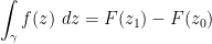
We now come to perhaps the most central theorem in complex analysis (save possibly for the fundamental theorem of calculus), namely Cauchy’s theorem, which allows one to compute a large number of contour integrals even without knowing any explicit antiderivative of
. There are many forms and variants of Cauchy’s theorem. To give one such version, we need the basic topological notion of a homotopy:
Definition 1 (Homotopy) Let
be an open subset of
, and let
,
be two curves in
.
- (i) If
have the same initial point
and terminal point
, we say that
and
are homotopic with fixed endpoints in
if there exists a continuous map
such that
and
for all
, and such that
and
for all
.
- (ii) If
are closed (but possibly with different initial points), we say that
and
are homotopic as closed curves in
if there exists a continuous map
such that
and
for all
, and such that
for all
.
- (iii) If
and
are curves with the same initial point and same terminal point, we say that
and
are homotopic with fixed endpoints up to reparameterisation in
if there is a reparameterisation
of
which is homotopic with fixed endpoints in
to a reparameterisation
of
.
- (iv) If
and
are closed curves, we say that
and
are homotopic as closed curves up to reparameterisation in
if there is a reparameterisation
of
which is homotopic as closed curves in
to a reparameterisation
of
.
In the first two cases, the map
will be referred to as a homotopy from
to
, and we will also say that
can be continously deformed to
(either with fixed endpoints, or as closed curves).
Example 2 If
is a convex set, that is to say that
whenever
and
, then any two curves
from one point
to another
are homotopic, by using the homotopy
For a similar reason, in a convex open set
, any two closed curves will be homotopic to each other as closed curves.
Exercise 3 Let
be an open subset of
.
- (i) Prove that the property of being homotopic with fixed endpoints in
is an equivalence relation.
- (ii) Prove that the property of being homotopic as closed curves in
is an equivalence relation.
- (iii) If
,
are closed curves with the same initial point, show that
is homotopic to
as closed curves up to reparameterisation if and only if
is homotopic to
with fixed endpoints for some closed curve
with the same initial point as
or
up to reparameterisation.
- (iv) Define a point in
to be a curve
of the form
for some
and all
. Let
be a closed curve in
. Show that
is homotopic with fixed endpoints to a point in
if and only if
is homotopic as a closed curve to a point in
. (In either case, we will call
homotopic to a point, null-homotopic, or contractible to a point in
.)
- (v) If
are curves with the same initial point and the same terminal point, show that
is homotopic to
with fixed endpoints in
if and only if
is homotopic to a point in
.
- (vi) If
is connected, and
are any two curves in
, show that there exists a continuous map
such that
and
for all
. Thus the notion of homotopy becomes rather trivial if one does not fix the endpoints or require the curve to be closed.
- (vii) Show that if
is a reparameterisation of
, then
and
are homotopic with fixed endpoints in U.
- (viii) Prove that the property of being homotopic with fixed endpoints in
up to reparameterisation is an equivalence relation.
- (ix) Prove that the property of being homotopic as closed curves in
up to reparameterisation is an equivalence relation.
We can then phrase Cauchy’s theorem as an assertion that contour integration on holomorphic functions is a homotopy invariant. More precisely:
Theorem 4 (Cauchy’s theorem) Let
be an open subset of
, and let
be holomorphic.
- (i) If
and
are rectifiable curves that are homotopic in
with fixed endpoints up to reparameterisation, then
- (ii) If
and
are closed rectifiable curves that are homotopic in
as closed curves up to reparameterisation, then
This version of Cauchy’s theorem is particularly useful for applications, as it explicitly brings into play the powerful technique of contour shifting, which allows one to compute a contour integral by replacing the contour with a homotopic contour on which the integral is easier to either compute or integrate. This formulation of Cauchy’s theorem also highlights the close relationship between contour integrals and the algebraic topology of the complex plane (and open subsets thereof). Setting
to be a point, we obtain an important special case of Cauchy’s theorem (which is in fact equivalent to the full theorem):
Corollary 5 (Cauchy’s theorem, again) Let
be an open subset of
, and let
be holomorphic. Then for any closed rectifiable curve
in
that is contractible in
to a point, one has
.
Exercise 6 Show that Theorem 4 and Corollary 5 are logically equivalent.
An important feature to note about Cauchy’s theorem is the global nature of its hypothesis on . The conclusion of Cauchy’s theorem only involves the values of a function
on the images of the two curves
. However, in order for the hypotheses of Cauchy’s theorem to apply, the function
must be holomorphic not only on the images on
, but on an open set
that is large enough (and sufficiently free of “holes”) to support a homotopy between the two curves. This point can be emphasised through the following fundamental near-counterexample to Cauchy’s theorem:
Example 7 (Key example) Let
, and let
be the holomorphic function
. Let
be the closed unit circle contour
. Direct calculation shows that
As a consequence of this and Cauchy’s theorem, we conclude that the contour
is not contractible to a point in
; note that this does not contradict Example 2 because
is not convex. Thus we see that the lack of holomorphicity (or singularity) of
at the origin can be “blamed” for the non-vanishing of the integral of
on the closed contour
, even though this contour does not come anywhere near the origin. Thus we see that the global behaviour of
, not just the behaviour in the local neighbourhood of
, has an impact on the contour integral.
One can of course rewrite this example to involve non-closed contours instead of closed ones. For instance, if we letdenote the half-circle contours
and
, then
are both contours in
from
to
, but one has
whereas
In order for this to be consistent with Cauchy’s theorem, we conclude that
and
are not homotopic in
(even after reparameterisation).
In the specific case of functions of the form , or more generally
for some point
and some
that is holomorphic in some neighbourhood of
, we can quantify the precise failure of Cauchy’s theorem through the Cauchy integral formula, and through the concept of a winding number. These turn out to be extremely powerful tools for understanding both the nature of holomorphic functions and the topology of open subsets of the complex plane, as we shall see in this and later notes.
Previous set of notes: Notes 1. Next set of notes: Notes 3.
Having discussed differentiation of complex mappings in the preceding notes, we now turn to the integration of complex maps. We first briefly review the situation of integration of (suitably regular) real functions of one variable. Actually there are three closely related concepts of integration that arise in this setting:
- (i) The signed definite integral
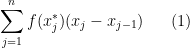
, which is usually interpreted as the Riemann integral (or equivalently, the Darboux integral), which can be defined as the limit (if it exists) of the Riemann sums
where
is some partition of
,
is an element of the interval
, and the limit is taken as the maximum mesh size
goes to zero (this can be formalised using the concept of a net). It is convenient to adopt the convention that
for
; alternatively one can interpret
as the limit of the Riemann sums (1), where now the (reversed) partition
goes leftwards from
to
, rather than rightwards from
to
.
- (ii) The unsigned definite integral
, usually interpreted as the Lebesgue integral. The precise definition of this integral is a little complicated (see e.g. this previous post), but roughly speaking the idea is to approximate
by simple functions
for some coefficients
and sets
, and then approximate the integral
by the quantities
, where
is the Lebesgue measure of
. In contrast to the signed definite integral, no orientation is imposed or used on the underlying domain of integration, which is viewed as an “undirected” set
.
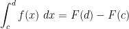
- (iii) The indefinite integral or antiderivative
, defined as any function
whose derivative
exists and is equal to
on
. Famously, the antiderivative is only defined up to the addition of an arbitrary constant
, thus for instance
.
There are some other variants of the above integrals (e.g. the Henstock-Kurzweil integral, discussed for instance in this previous post), which can handle slightly different classes of functions and have slightly different properties than the standard integrals listed here, but we will not need to discuss such alternative integrals in this course (with the exception of some improper and principal value integrals, which we will encounter in later notes).
The above three notions of integration are closely related to each other. For instance, if is a Riemann integrable function, then the signed definite integral and unsigned definite integral coincide (when the former is oriented correctly), thus
and
If is continuous, then by the fundamental theorem of calculus, it possesses an antiderivative
, which is well defined up to an additive constant
, and
for any , thus for instance
and
.
All three of the above integration concepts have analogues in complex analysis. By far the most important notion will be the complex analogue of the signed definite integral, namely the contour integral , in which the directed line segment from one real number
to another
is now replaced by a type of curve in the complex plane known as a contour. The contour integral can be viewed as the special case of the more general line integral
, that is of particular relevance in complex analysis. There are also analogues of the Lebesgue integral, namely the arclength measure integrals
and the area integrals
, but these play only an auxiliary role in the subject. Finally, we still have the notion of an antiderivative
(also known as a primitive) of a complex function
.
As it turns out, the fundamental theorem of calculus continues to hold in the complex plane: under suitable regularity assumptions on a complex function and a primitive
of that function, one has
whenever is a contour from
to
that lies in the domain of
. In particular, functions
that possess a primitive must be conservative in the sense that
for any closed contour. This property of being conservative is not typical, in that “most” functions
will not be conservative. However, there is a remarkable and far-reaching theorem, the Cauchy integral theorem (also known as the Cauchy-Goursat theorem), which asserts that any holomorphic function is conservative, so long as the domain is simply connected (or if one restricts attention to contractible closed contours). We will explore this theorem and several of its consequences in the next set of notes.
Read the rest of this entry »
In Notes 1, we approached multiplicative number theory (the study of multiplicative functions and their relatives) via elementary methods, in which attention was primarily focused on obtaining asymptotic control on summatory functions
and logarithmic sums
. Now we turn to the complex approach to multiplicative number theory, in which the focus is instead on obtaining various types of control on the Dirichlet series
, defined (at least for
of sufficiently large real part) by the formula
These series also made an appearance in the elementary approach to the subject, but only for real that were larger than
. But now we will exploit the freedom to extend the variable
to the complex domain; this gives enough freedom (in principle, at least) to recover control of elementary sums such as
or
from control on the Dirichlet series. Crucially, for many key functions
of number-theoretic interest, the Dirichlet series
can be analytically (or at least meromorphically) continued to the left of the line
. The zeroes and poles of the resulting meromorphic continuations of
(and of related functions) then turn out to control the asymptotic behaviour of the elementary sums of
; the more one knows about the former, the more one knows about the latter. In particular, knowledge of where the zeroes of the Riemann zeta function
are located can give very precise information about the distribution of the primes, by means of a fundamental relationship known as the explicit formula. There are many ways of phrasing this explicit formula (both in exact and in approximate forms), but they are all trying to formalise an approximation to the von Mangoldt function
(and hence to the primes) of the form
where the sum is over zeroes (counting multiplicity) of the Riemann zeta function
(with the sum often restricted so that
has large real part and bounded imaginary part), and the approximation is in a suitable weak sense, so that
for suitable “test functions” (which in practice are restricted to be fairly smooth and slowly varying, with the precise amount of restriction dependent on the amount of truncation in the sum over zeroes one wishes to take). Among other things, such approximations can be used to rigorously establish the prime number theorem
as , with the size of the error term
closely tied to the location of the zeroes
of the Riemann zeta function.
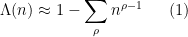
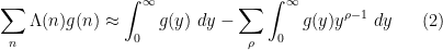
The explicit formula (1) (or any of its more rigorous forms) is closely tied to the counterpart approximation
for the Dirichlet series of the von Mangoldt function; note that (4) is formally the special case of (2) when
. Such approximations come from the general theory of local factorisations of meromorphic functions, as discussed in Supplement 2; the passage from (4) to (2) is accomplished by such tools as the residue theorem and the Fourier inversion formula, which were also covered in Supplement 2. The relative ease of uncovering the Fourier-like duality between primes and zeroes (sometimes referred to poetically as the “music of the primes”) is one of the major advantages of the complex-analytic approach to multiplicative number theory; this important duality tends to be rather obscured in the other approaches to the subject, although it can still in principle be discernible with sufficient effort.
More generally, one has an explicit formula
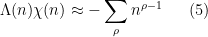
for any (non-principal) Dirichlet character , where
now ranges over the zeroes of the associated Dirichlet
-function
; we view this formula as a “twist” of (1) by the Dirichlet character
. The explicit formula (5), proven similarly (in any of its rigorous forms) to (1), is important in establishing the prime number theorem in arithmetic progressions, which asserts that
as , whenever
is a fixed primitive residue class. Again, the size of the error term
here is closely tied to the location of the zeroes of the Dirichlet
-function, with particular importance given to whether there is a zero very close to
(such a zero is known as an exceptional zero or Siegel zero).
While any information on the behaviour of zeta functions or -functions is in principle welcome for the purposes of analytic number theory, some regions of the complex plane are more important than others in this regard, due to the differing weights assigned to each zero in the explicit formula. Roughly speaking, in descending order of importance, the most crucial regions on which knowledge of these functions is useful are
- The region on or near the point
.
- The region on or near the right edge
of the critical strip
.
- The right half
of the critical strip.
- The region on or near the critical line
that bisects the critical strip.
- Everywhere else.
For instance:
- We will shortly show that the Riemann zeta function
has a simple pole at
with residue
, which is already sufficient to recover much of the classical theorems of Mertens discussed in the previous set of notes, as well as results on mean values of multiplicative functions such as the divisor function
. For Dirichlet
-functions, the behaviour is instead controlled by the quantity
discussed in Notes 1, which is in turn closely tied to the existence and location of a Siegel zero.
- The zeta function is also known to have no zeroes on the right edge
of the critical strip, which is sufficient to prove (and is in fact equivalent to) the prime number theorem. Any enlargement of the zero-free region for
into the critical strip leads to improved error terms in that theorem, with larger zero-free regions leading to stronger error estimates. Similarly for
-functions and the prime number theorem in arithmetic progressions.
- The (as yet unproven) Riemann hypothesis prohibits
from having any zeroes within the right half
of the critical strip, and gives very good control on the number of primes in intervals, even when the intervals are relatively short compared to the size of the entries. Even without assuming the Riemann hypothesis, zero density estimates in this region are available that give some partial control of this form. Similarly for
-functions, primes in short arithmetic progressions, and the generalised Riemann hypothesis.
- Assuming the Riemann hypothesis, further distributional information about the zeroes on the critical line (such as Montgomery’s pair correlation conjecture, or the more general GUE hypothesis) can give finer information about the error terms in the prime number theorem in short intervals, as well as other arithmetic information. Again, one has analogues for
-functions and primes in short arithmetic progressions.
- The functional equation of the zeta function describes the behaviour of
to the left of the critical line, in terms of the behaviour to the right of the critical line. This is useful for building a “global” picture of the structure of the zeta function, and for improving a number of estimates about that function, but (in the absence of unproven conjectures such as the Riemann hypothesis or the pair correlation conjecture) it turns out that many of the basic analytic number theory results using the zeta function can be established without relying on this equation. Similarly for
-functions.
Remark 1 If one takes an “adelic” viewpoint, one can unite the Riemann zeta function
and all of the
-functions
for various Dirichlet characters
into a single object, viewing
as a general multiplicative character on the adeles; thus the imaginary coordinate
and the Dirichlet character
are really the Archimedean and non-Archimedean components respectively of a single adelic frequency parameter. This viewpoint was famously developed in Tate’s thesis, which among other things helps to clarify the nature of the functional equation, as discussed in this previous post. We will not pursue the adelic viewpoint further in these notes, but it does supply a “high-level” explanation for why so much of the theory of the Riemann zeta function extends to the Dirichlet
-functions. (The non-Archimedean character
and the Archimedean character
behave similarly from an algebraic point of view, but not so much from an analytic point of view; as such, the adelic viewpoint is well suited for algebraic tasks (such as establishing the functional equation), but not for analytic tasks (such as establishing a zero-free region).)
Roughly speaking, the elementary multiplicative number theory from Notes 1 corresponds to the information one can extract from the complex-analytic method in region 1 of the above hierarchy, while the more advanced elementary number theory used to prove the prime number theorem (and which we will not cover in full detail in these notes) corresponds to what one can extract from regions 1 and 2.
As a consequence of this hierarchy of importance, information about the function away from the critical strip, such as Euler’s identity
or equivalently
or the infamous identity
which is often presented (slightly misleadingly, if one’s conventions for divergent summation are not made explicit) as
are of relatively little direct importance in analytic prime number theory, although they are still of interest for some other, non-number-theoretic, applications. (The quantity does play a minor role as a normalising factor in some asymptotics, see e.g. Exercise 28 from Notes 1, but its precise value is usually not of major importance.) In contrast, the value
of an
-function at
turns out to be extremely important in analytic number theory, with many results in this subject relying ultimately on a non-trivial lower-bound on this quantity coming from Siegel’s theorem, discussed below the fold.
For a more in-depth treatment of the topics in this set of notes, see Davenport’s “Multiplicative number theory“.
Recent Comments