
One theme in this course will be the central nature played by the gaussian random variables 
One way to exploit this algebraic structure is to continuously deform the variance 


At present, we have not completely specified what 

We will begin with one-dimensional Brownian motion, but it is a simple matter to extend the process to higher dimensions. In particular, we can define Brownian motion on vector spaces of matrices, such as the space of 
— 1. Formal construction of Brownian motion —
We begin with constructing one-dimensional Brownian motion. We shall model this motion using the machinery of Wiener processes:
Definition 1 (Wiener process) Let
, and let
be a set of times containing
with initial position
is a collection
of real random variables
, with the following properties:
- (i)
.
- (ii) Almost surely, the map
- (iii) For every
in
has the distribution of
. (In particular,
for every
.)
- (iv) For every
in
for
are jointly independent.
If
then we say that
Remark 2 Collections of random variables
Remark 3 In the case of discrete Wiener processes, the continuity requirement (ii) is automatic. For continuous Wiener processes, there is a minor technical issue: the event that
, such that
(with the product
-algebra, of course).
Remark 4 One can clearly normalise the initial position
for each
We shall abuse notation somewhat and identify continuous Wiener processes with Brownian motion in our informal discussion, although technically the former is merely a model for the latter. To emphasise this link with Brownian motion, we shall often denote continuous Wiener processes as 

It is not yet obvious that Wiener processes exist, and to what extent they are unique. The situation is easily clarified though for discrete processes:
Proposition 5 (Discrete Brownian motion) Let
containing
. Then (after extending the sample space if necessary) there exists a Wiener process
with base point
Proof: As 

Let 

for all 
Conversely, if 


Now we pass from the discrete case to the continuous case.
Proposition 6 (Continuous Brownian motion) Let
with base point
Proof: The uniqueness claim follows by the same argument used to prove the uniqueness component of Proposition 5, so we just prove existence here. The iterative construction we give here is somewhat analogous to that used to create self-similar fractals, such as the Koch snowflake. (Indeed, Brownian motion can be viewed as a probabilistic analogue of a self-similar fractal.)
The idea is to create a sequence of increasingly fine discrete Brownian motions, and then to take a limit. Proposition 5 allows one to create each individual discrete Brownian motion, but the key is to couple these discrete processes together in a consistent manner.
Here’s how. We start with a discrete Wiener process 

for 


Next, we extend the process further to the denser set of times 
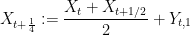
where 


Iterating this procedure a countable number of times, we obtain a collection of discrete Wiener processes 

Now we establish a Hölder continuity property. Let 


for some absolute constants 


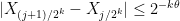
for all but finitely many 

![{[0,T]}](https://s0.wp.com/latex.php?latex=%7B%5B0%2CT%5D%7D&bg=ffffff&fg=000000&s=0&c=20201002)
As the dyadic rationals are dense in 


Remark 7 One could also have used the Kolmogorov extension theorem to establish the limit.
Exercise 8 Let
, that the map
, then the map
Show also that the map
Remark 9 In the above constructions, the initial position
is itself a random variable. Indeed, one can simply set
where
, but is instead the convolution of the law of
.

— 2. Connection with random walks —
We saw how to construct Brownian motion as a limit of discrete Wiener processes, which were partial sums of independent gaussian random variables. The central limit theorem (see Notes 2) allows one to interpret Brownian motion in terms of limits of partial sums of more general independent random variables, otherwise known as (independent) random walks.
Definition 10 (Random walk) Let
be a real random variable, let
be a time step. We define a discrete random walk with initial position
and step distribution
) to be a process
defined by
where
are iid copies of

Example 11 From the proof of Proposition 5, we see that a discrete Wiener process on
with initial position
. Another basic example is simple random walk, in which
times a signed Bernoulli variable, thus we have
, where the signs
are unbiased and are jointly independent in
Exercise 12 (Central limit theorem) Let
be a real random variable with mean zero and variance
be a process formed by starting with a random walk
with initial position
, and then extending to other times in
for all
and
. Show that as
, the process

— 3. Connection with the heat equation —
Let 


Lemma 13 (Equation of motion) For all times
, we have
where
is the second derivative of
. In particular,

Proof: We work from first principles. It suffices to show for fixed

as 


Write 

We take expectations. Since 


Now observe that 
Exercise 14 Complete the proof of the lemma by considering negative values of
. Also, use the fact that
and
are continuous in
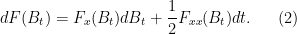
Remark 15 In the language of Ito calculus, we can write (1) as
Here,
, and
and third moment
. This is a special case of Ito’s formula. It should be compared against the chain rule
when
and
, with the understanding that all terms that are
Let 


for any Schwartz function
in the sense of (tempered) distributions (see e.g. my earlier notes on this topic). In other words, 
From the theory of PDE (e.g. from Fourier analysis, see Exercise 38 of these notes) one can solve the (distributional) heat equation with this initial data to obtain the unique solution

Of course, this is also the density function of 
Remark 16 Because we considered a Wiener process with a deterministic initial position
We have related one-dimensional Brownian motion to the one-dimensional heat equation, but there is no difficulty establishing a similar relationship in higher dimensions. In a vector space 


where 
Exercise 17 If
whenever
is smooth with all derivatives bounded, where
is the Laplacian of


A simple but fundamental observation is that 


This is ultimately because the 
Remark 18 One can also relate variable-coefficient heat equations to variable-coefficient Brownian motion
is now only proportional to
Exercise 19 Let
be a real random variable of mean zero and variance
where
- Show that each
- Show that
as
.
- If
where
is the Ornstein-Uhlenbeck operator
Conclude that the density function
of
where the adjoint operator
is given by
- Show that the only probability density function
is the Gaussian
; furthermore, show that
for all probability density functions


Remark 20 The heat kernel
in
dimensions is absolutely integrable in time away from the initial time
, but becomes divergent in dimension
. This causes the qualitative behaviour of Brownian motion
to be rather different in the two regimes. For instance, in dimensions
as
Brownian motion is recurrent: for each
, one almost surely has
for infinitely many
at arbitrarily large times, but does not visit
— 4. Dyson Brownian motion —
The space 


where 


Now that one has this indentification, for each Hermitian matrix 


Given any Hermitian matrix 

in the Weyl cone. We abbreviate 

For 
The stochastic dynamics of this evolution can be described by Dyson Brownian motion:
Theorem 21 (Dyson Brownian motion) Let
, and let
be as above. Then we have
for all
, where
, and
are iid copies of
which are jointly independent of
, and the error term
is the sum of two terms, one of which has
norm
in the limit

Using the language of Ito calculus, one usually views

that shows that the eigenvalues
Proof: Fix 

Almost surely, 


which by dyadic decomposition implies the finite negative second moment

Let 

and

where 

(One can obtain a more exact third Hadamard variation formula if desired, but it is messy and will not be needed here.) A Taylor expansion now gives the bound

provided that one is in the regime
(in order to keep the eigenvalue gap at least 

we can instead use the Weyl inequalities to bound 


Now we take advantage of the unitary invariance of the Gaussian unitary ensemble (that is, that 


where 


are acceptable error terms. But the first term has mean zero and is bounded by 


Remark 22 Interestingly, one can interpret Dyson Brownian motion in a different way, namely as the motion of
after one conditions the
In the previous section, we saw how a Wiener process led to a PDE (the heat flow equation) that could be used to derive the probability density function for each component
Exercise 23 Let
where
is the adjoint Dyson operator
If we let
denote the density function
of
at time
, deduce the Dyson partial differential equation
(in the sense of distributions, at least, and on the interior of
), where
is the Dyson operator


The Dyson partial differential equation (8) looks a bit complicated, but it can be simplified (formally, at least) by introducing the Vandermonde determinant
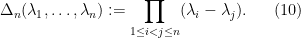
Exercise 24 Show that (10) is the determinant of the matrix
, and is also the sum
.
Note that this determinant is non-zero on the interior of the Weyl chamber
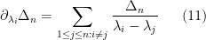
which can be used to cancel off the second term in (9). Indeed, we have
Exercise 25 Let
in this interior. Show that
obeys the linear heat equation
in the interior of
for distinct
. Equivalently, you may need to first establish that the Vandermonde determinant is a harmonic function.)


Let 
Now suppose that the initial matrix 


Using the fundamental solution for the heat equation in

By the Leibniz formula for determinants, we can express the sum here as a determinant of the matrix
Applying (12), we conclude
Theorem 26 (Johansson formula) Let
where
of
on

This formula is given explicitly in this paper of Johansson, who cites this paper of Brézin and Hikami as inspiration. This formula can also be proven by a variety of other means, for instance via the Harish-Chandra formula. (One can also check by hand that (13) satisfies the Dyson equation (8).)
We will be particularly interested in the case when 


Exercise 27 Show that as
and
locally uniformly in
vanishes and so can be treated by the (smooth) factor theorem.)


From the above exercise, we conclude the fundamental Ginibre formula

for the density function for the spectrum
This formula can be derived by a variety of other means; we sketch one such way below.
Exercise 28 For this exercise, assume that it is known that (14) is indeed a probability distribution on the Weyl chamber
by an unspecified normalisation factor depending only on
be drawn at random using the distribution (14), and let
be drawn at random from Haar measure on
. Show that the probability density function of
at a matrix
for some constant
. (Hint: use unitary invariance to reduce to the case when
and consider what
).)
Conclude that (14) must be the probability density function of the spectrum of a GUE matrix.
Exercise 29 Verify by hand that the self-similar extension
of the function (14) obeys the Dyson PDE (8). Why is this consistent with (14) being the density function for the spectrum of GUE?

Remark 30 Similar explicit formulae exist for other invariant ensembles, such as the gaussian orthogonal ensemble GOE and the gaussian symplectic ensemble GSE. One can also replace the exponent in density functions such as
with more general expressions than quadratic expressions of

55 comments
Comments feed for this article
18 January, 2010 at 7:02 pm
Joshua Batson
I think last display in the proof of prop. 3 should be not
not  .
.
[Corrected, thanks – T.]
18 January, 2010 at 7:36 pm
Anonymous
Wonderful post. Everything looks different in your hands.
Thank you Prof. Tao.
19 January, 2010 at 8:32 am
Tim vB
Dear Terry,
marvelous lecture notes, thanks for making them public!
On a side note I would like to mention that it can be fun to code a discretization scheme for stochastic differential equations aka a simulation of a stochastic process, in order to solve the associated partial differential equation. It’s one thing to prove that it can be done, but it can be fun too to look at some specific examples and compare the results of the simulation with numerical or analytical results that you get from the partial differential equation.
That’s off topic with regard to your class of course, but maybe some of your students would like to takle that in their spare time, if they have any :-)
(I think that is still an active research topic, used e.g. for PDE with complicated domains/boundaries and boundary conditions, but I’ve been out of the field for years).
BTW: Do you use computer simulations in the class?
19 January, 2010 at 4:13 pm
David Speyer
Possible typo: In the paragraph beginning “Now we establish a Hölder continuity property. Let theta be any exponent between 0 and 2”, I think that 2 should be 1/2.
These are great notes; I am starting to understand what a random walk is.
19 January, 2010 at 5:43 pm
Anonymous
There are eleven “Formula does not parse” errors. I’m using Firefox 3.5.7. The first one is in the def of Wiener Process:
A (one-dimensional) Wiener process on {\Sigma} with initial position {\mu} is a collection {(X_t)_{t \in \Sigma}} of real random …
Here, {(X_t)_{t \in \Sigma}} does not parse.
19 January, 2010 at 7:22 pm
Jonathan Vos Post
I also get eleven “Formula does not parse” errors, using Firefox 3.5.7.
20 January, 2010 at 5:53 am
Tim vB
That does not seem to be a problem of the browser, I’m using Firefox 3.5.7 as well and all formulas are rendered without any problems, but I see them as embedded png graphics.
20 January, 2010 at 12:09 pm
Américo Tavares
A few hours ago I also got the same errors but now all formulas are OK. (I’m using IE).
25 January, 2010 at 7:45 pm
solrize
This post and and the post of a few days ago reviewing probability theory are great. It’s important material that I’ve been wanting to understand for quite a while. I’ve looked at some elementary books that were muddled and left out all the interesting stuff, and I’ve looked at some more advanced books that had way too much assumed background for me (ex-undergrad math major) to understand. These posts of yours are at a level that I think I can make my way through if I work at it, and which appear to demystify the subject. That’s hard to find. Thanks!!!!
28 January, 2010 at 11:30 am
Doug
Hi Terrence,
I have found a discussion of the LOUIS BACHELIER 1900 thesis “THEORIE DE LA SPECULATION” with Brownian motion applied to the stock market [Mathematical Finance, Vol.10, No.3 (July 2000), 341–353].
The appendix of this paper includes the faculty report by Appell, Poincare, J. Boussinesq.
This report is somewhat critical of the institution used, but praises the originality of this type of probability theory [p 349]:
“The manner in which M. Bachelier deduces Gauss’s law is very original, and all the more interesting in that his reasoning can be extended with a few changes to the theory of errors. … In fact, the author makes a comparison with the analytic theory of heat flow. A bit of thought shows that the analogy is real and the comparison is legitimate. The reasoning of Fourier, almost without change, is applicable to this problem so different from the one for which it was originally created. It is regrettable that M. Bachelier did not develop this part of his thesis further. He could have entered into the details of Fourier’s analysis. He did, however, say enough about it to justify Gauss’s law and to foresee cases where it would no longer hold.
Once Gauss’s law is established, one can easily deduce certain consequences susceptible to experimental verification. Such an example is the relation between the value of an option and the deviation from the underlying. One should not expect a very exact verification. The principle of the mathematical expectation holds in the sense that, if it were violated, there would always be people who would act so as to re-establish it and they would eventually notice this. But they would only notice it if the deviations were considerable. The verification, then, can only be gross. The author of the thesis gives statistics where this happens in a very satisfactory manner.
…
In summary, we are of the opinion that there is reason to authorize M. Bachelier tohave his thesis printed and to submit it.”
1 February, 2010 at 4:53 pm
Anonymous
Dear Prof. Tao, there seem to be two typos
between Exercise 4 and Remark 8: “dmiensional”, “ebcause”.
[Corrected, thanks – T.]
2 February, 2010 at 1:34 pm
254A, Notes 4: The semi-circular law « What’s new
[…] transform method, together with a third (heuristic) method based on Dyson Brownian motion (Notes 3b). In the next set of notes we shall also study the free probability method, and in the set of notes […]
18 February, 2010 at 11:04 am
Ben
Hi Terry,
I think there’s a link problem. These notes, Notes 3b: Brownian motion and Dyson Brownian motion seem to be the the same as the notes on eigenvalues, Notes 3b (and don’t mention Dyson’s BM at all). I was able to access the notes yesterday but not today. I’m not sure if this problem is specific to me.
[Whoops, this was caused by a bad edit on my part. Corrected, thanks. -T.]
23 February, 2010 at 12:24 am
Mio
In fractal construction, in order for to have variance
  , shouldn’t
  have variance 1/2 and not 1/4 (same for
  below, 1/4 instead of 1/8)?
23 February, 2010 at 8:03 am
Terence Tao
Well, already has a variance of
  , so one only needs an additional variance of
  from
from  to balance it.
23 February, 2010 at 8:14 am
Mio
Oops, sorry. Thanks for a great lecture.
23 February, 2010 at 8:15 am
Ben
23 February, 2010 at 3:43 pm
Alex Bloemendal
Great lecture. The proof of the Ginibre formula (12) for the eigenvalue density of a GUE matrix given in Dyson’s original paper is perhaps even simpler than the one you present. Dyson adds the Ornstein-Uhlenbeck restoring term to the matrix entry processes, which just adds the same term to the induced eigenvalue processes. The matrix evolution then has GUE as its unique stationary distribution; on the other hand, we can obtain the corresponding stationary distribution for the eigenvalues as the unique probability density that is a stationary solution of the resulting modified Dyson PDE (6), which is easily seen to be (12).
I do realize this comment boils down to Exercise 11, but thought it was worth mentioning anyway — because the argument is physically compelling, and because you did introduce the Ornstein-Uhlenbeck process.
By the way, while Exercise 5 is internally consistent, your definition of Ornstein-Uhlenbeck is off from the usual one by a time-change — it has the wrong quadratic variation! I guess this is the source of the extra factor that appears in the definition of the generator
  (which, incidentally, is not self-adjoint!).
23 February, 2010 at 10:50 pm
Terence Tao
Thanks for the corrections and comments! It’s true that the Ornstein-Uhlenbeck approach is slightly more efficient to get the Ginibre formula, but I like the heat equation approach as it also gives the Johansson formula quite easily. Though of course, as you say, the two approaches are simply rescalings of each other, so the differences are minor.
23 February, 2010 at 5:20 pm
Alex Bloemendal
A comment regarding Remark 9:
Two-dimensional Brownian motion almost surely never hits a given point
  after time 0. My favourite proof uses the interpretation of certain harmonic functions as hitting probabilities, together with the form of the Green’s function of the 2-d Laplacian, to establish the following fact. Surround
  with concentric circles
  of radii
  for all
  ; then the sequence of indices of the successive circles hit by
  (ignoring immediate repetition) forms a simple random walk on
  ! In particular,
  must return to
  at arbitrarily large times, in between any two of which it can visit only finitely many
  ‘s. (This argument actually establishes neighbourhood recurrence as well, since
  must also hit each small circle at arbitrarily large times.)
Like everyone here, I seriously appreciate your wonderful notes and all the time you spend interacting with your readers.
23 February, 2010 at 10:02 pm
254A, Notes 6: Gaussian ensembles « What’s new
[…] have already shown using Dyson Brownian motion in Notes 3b that we have the Ginibre […]
5 March, 2010 at 1:47 pm
254A, Notes 7: The least singular value « What’s new
[…] so we expect each to have magnitude about . This, together with the Hoeffman-Wielandt inequality (Notes 3b) means that we expect to differ by from . In principle, this gives us asymptotic universality on […]
12 March, 2010 at 6:37 pm
Anonymous
Dear Prof. Tao,
Can we define Brownian motion on an infinite dimensional vector space?
a second question :we know that has mean zero and variance is
  therefore
  has variance 1. but why do we have
  be of
be of  ?
?
thanks
14 March, 2010 at 12:17 am
Terence Tao
Well, there are no non-trivial unitarily invariant probability distributions on a Hilbert space (each coordinate would almost surely be zero), so one has to give up either isotropy or finite norm in order to have a meaningful infinite-dimensional Brownian motion. Of course, once one gives up either, one can certainly define Brownian-like motions (e.g. by picking an orthonormal basis and placing an independent weighted copy of Brownian motion in each coordinate).
13 March, 2010 at 9:42 pm
student
Dear Prof. Tao,
We can consider Brownian motion as a random variable from a probability space to![C([0,T]\rightarrow {\mathbb R})](https://s0.wp.com/latex.php?latex=C%28%5B0%2CT%5D%5Crightarrow+%7B%5Cmathbb+R%7D%29&bg=ffffff&fg=545454&s=0&c=20201002)
Do we have a Markov process which can be considered as a random variable from a probability space to![C^{\infty}([0,T]\rightarrow {\mathbb R})](https://s0.wp.com/latex.php?latex=C%5E%7B%5Cinfty%7D%28%5B0%2CT%5D%5Crightarrow+%7B%5Cmathbb+R%7D%29&bg=ffffff&fg=545454&s=0&c=20201002)
thanks
14 March, 2010 at 12:22 am
Terence Tao
It depends a little on how one defines the “present state” of the system, but using a naive notion of the Markov property, the right-derivative would need to be independent of the left-derivative at time t when the position at t is fixed. But for a function, these two derivatives are equal, and thus must be determined completely by the position at t. This suggests to me (from the Picard uniqueness theorem) that the only processes of this type are the deterministic ones, though there is the loophole that the derivative is not required to depend in a Lipschitz manner on the position.
14 March, 2010 at 6:22 am
beginner
but the same argument should apply the continuous case as well. on the other hand we know that Brownian motion is a Markov process and has continuous paths. Maybe I am missing a point.
thanks
14 March, 2010 at 10:15 am
Terence Tao
Continuous paths need not have left or right derivatives.
30 January, 2011 at 1:23 pm
Carl Mueller
Usually the sigma-fields are assumed to be right continuous, meaning that the current state contains information about the infinitesimal future. So the right hand derivative (if it existed) would be part of the current state.
4 April, 2010 at 7:57 am
Dyson’s Brownian Motion « Rochester Probability Blog
[…] Dyson’s Brownian Motion Filed under: Uncategorized — carl0mueller @ 3:57 pm Tags: background See also: Tao’s blog on Dyson’s Brownian motion […]
27 January, 2011 at 2:15 pm
Minyu
Hi, Professor Tao:
There is a constant missing in the Ginibre formula and Exercise 9. It’s the reciprocal of a product of some factorials…
[Corrected, thanks – T.]
30 January, 2011 at 12:52 pm
yucao
Is it possible to extend the Brownian motion on the whole
  , i.e.
  ?
?
15 July, 2011 at 9:59 am
Dyson Brownian Motion | Research Notebook
[…] main source for the material in this post is Terry Tao‘s set of lecture notes on Random Matrix Theory, though I also used Mehta (2004) and Anderson, Guinnet and Zeitouni (2009) as […]
21 August, 2011 at 9:36 am
On Understanding Probability Puzzles | Nair Research Notes
[…] by , from an experimental point of view. The formal construction for the Brownian motion can be found here for example. And you will get a good historical perspective of the Brownian motion here. One of the […]
18 November, 2011 at 2:38 am
Diffusion in Ehrenfest wind-tree model « Disquisitiones Mathematicae
[…] the “justification” of the word “abnormal” comes by comparison with Brownian motion and/or central limit theorem: once we know that the diffusion is “sublinear” (maybe […]
18 January, 2012 at 12:12 pm
Anonymous
Hi prof. Tau,
Thanks for these great notes!
Maybe this question is much too late, but I’d be very grateful for a reply. I’m used to think about the eigenvalues of the GUE as being subjected to a quadratic confining potential and mutual log repulsion: is there an easy way to understand the absence of the effect of the confining potential (which would give rise to a simple harmonic restoring force for each eigenvalue) in the formula for the Dyson Brownian motion, equation (5)?
Thanks for a great blog!
18 January, 2012 at 6:09 pm
Terence Tao
One can restore the confining potential by adding a term to the equation for
  , turning the Dyson Brownian motion to a Dyson Ornstein-Uhlenbeck process. This has the effect of keeping the variance of the matrix entries in the process constant, instead of growing linearly in time as is done here.
The two processes (normalised variance and non-normalised variance) can be easily rescaled to each other, so the choice of which one to use is basically a matter of taste.
1 May, 2012 at 10:52 am
alabair
I am amazed by the surprising number of knowledge that is difficult to me to digest. And by the way, I would like to hear about a white noise process. Good luck.
11 November, 2012 at 1:09 pm
A direct proof of the stationarity of the Dyson sine process under Dyson Brownian motion « What’s new
[…] of a Hermitian matrix under independent Brownian motion of its entries, and is discussed in this previous blog post. To cut a long story short, this stationarity tells us that the self-similar -point correlation […]
4 February, 2013 at 2:10 am
hera
Great lecture! Prof. Tao, do you have ideas to simulate the Dyson’s brownian motion ? I’d like to do a computer simulation with MATLAB, can you give me some ideas?
5 February, 2013 at 2:47 pm
Some notes on Bakry-Emery theory « What’s new
[…] is a stochastic process with initial probability distribution ; see for instance this previous blog post for more […]
8 February, 2013 at 5:47 pm
The Harish-Chandra-Itzykson-Zuber integral formula « What’s new
[…] motion (as well as the closely related formulae for the GUE ensemble), which were derived in this previous blog post. Both of these approaches can be found in several places in the literature (and I do not actually […]
24 April, 2014 at 12:39 am
Sticky Brownian Motion | Eventually Almost Everywhere
[…] 254A, Notes 3b: Brownian motion and Dyson Brownian motion (terrytao.wordpress.com) […]
25 December, 2014 at 3:31 pm
Ramis Movassagh
Dear Terry,
Thank you for the wonderful post (your posts are always a joy to read and learn from).
Shouldn’t Prop. 2 end with “…same distribution at X_t” instead of \mu?
Best, – Ramis
[Corrected, thanks – T.]
25 December, 2014 at 6:37 pm
Ramis Movassagh
Hi Terry, Same with Prop 3. Thanks for the great post.
cheers, -R
[Corrected, thanks – T.]
7 January, 2016 at 12:45 pm
Ito Calculus by peatar | wanikanidailyscience
[…] Warning: I don’t really know much about financial mathematics so if there are any economists around: Let me know about eventual mistakes. Sources: Links in the text and Terry Tao’s blog. […]
8 November, 2017 at 12:24 am
Student
Dear Professor Tao, has O(
 ) third moment, but the constant of the big order should be O(
 ). Upon doing the conditioning I think one should check
  has finite third moment, but how can I do that?
In the last part Theorem 6,
thanks
8 November, 2017 at 3:27 pm
Terence Tao
Actually, the third derivative scales like , so one only needs to control the second moment, not the third. The probability that two eigenvalues are within
  of each other is bounded by
  (this is because the Vandermonde determinant is
  ), where we allow implied constants to depend on
  . So the second moment is finite.
11 November, 2017 at 12:19 am
Student
By the independence of , product of two or three random variables will have zero expectation, so
 .
. be derived by direct computation? or there is some relation I need to use?
Can the term
The of Vandermonde determinant and the process is derived in Exercise 6 and Theorem 6.
Will Using it to discuss the gap between the eigenvalues lead to circular argument(because it is a part of proof of Theorem 6)?
11 November, 2017 at 9:50 am
Terence Tao
You are right, the third moment bound is a bit too strong. I have rewritten the argument to only claim the second moment bound (for one error term) and an L^1 bound (for the other error term), which still suffices.
29 May, 2018 at 9:30 am
246C notes 4: Brownian motion, conformal invariance, and SLE | What's new
[…] and complex Brownian motions exist from any base point or ; see e.g. this previous blog post for a construction. We have the following simple […]
24 August, 2020 at 4:37 pm
Yixuan Zhou
Dear Professor Tao, I want to ask whether we can take the derivatives of the eigenvalues when we are trying to prove the Dyson Brownian Motion’s equation. I know from a previous note you justified the smoothness when the matrix process that we obtained is smooth with respect to time. However, it is not clear to me that Hermitian matrix valued BM is smooth.
31 August, 2020 at 5:00 pm
Terence Tao
The eigenvalues of a DBM will not be classically differentiable, but one can still manipulate their time derivative by the usual tools of stochastic differential calculus (in particular Ito calculus).
14 September, 2020 at 3:13 pm
Student
Dear Professor Tao,
I have a question about the last part where we derive the Johansson formula. I don’t think I am understanding the argument of extending the probability density function symmetrically from the Weyl chamber to the whole space. The questions that lingers are, first what do you mean by extending a function symmetrically. And second, why would we sum up the different initial starting location if the eigenvalues should be non-crossing.
Thanks in advance!
[See https://en.wikipedia.org/wiki/Symmetric_function ]
6 February, 2021 at 4:43 am
Anonymous
Don’t the eigenvalues of a GUE sample lie on a disk of unit radius, i.e. Girko’s law?
[The circular law of Girko is for non-Hermitian random matrices such as the Ginibre ensemble, whereas the GUE ensemble (which shoudl not be confused with the Ginibre ensemble) is Hermitian. -T]