
In set theory, a function 


Generalisations of functions are also very useful in analysis. In our study of 


We have also seen (via the Lebesgue-Radon-Nikodym theorem) that locally integrable functions 


There is an even larger class of generalised functions that is very useful, particularly in linear PDE, namely the space of distributions, say on a Euclidean space 


If one shrinks the space of distributions slightly, to the space of tempered distributions (which is formed by enlarging dual class 
Of course, at the end of the day, one is usually not all that interested in distributions in their own right, but would like to be able to use them as a tool to study more classical objects, such as smooth functions. Fortunately, one can recover facts about smooth functions from facts about the (far rougher) space of distributions in a number of ways. For instance, if one convolves a distribution with a smooth, compactly supported function, one gets back a smooth function. This is a particularly useful fact in the theory of constant-coefficient linear partial differential equations such as 


It is this unusual and useful combination of both being able to pass from classical functions to generalised functions (e.g. by differentiation) and then back from generalised functions to classical functions (e.g. by convolution) that sets the theory of distributions apart from other competing theories of generalised functions, in particular allowing one to justify many formal calculations in PDE and Fourier analysis rigorously with relatively little additional effort. On the other hand, being defined by linear duality, the theory of distributions becomes somewhat less useful when one moves to more nonlinear problems, such as nonlinear PDE. However, they still serve an important supporting role in such problems as a “ambient space” of functions, inside of which one carves out more useful function spaces, such as Sobolev spaces, which we will discuss in the next set of notes.
— 1. Smooth functions with compact support —
In the rest of the notes we will work on a fixed Euclidean space 
A test function is any smooth, compactly supported function 

From analytic continuation one sees that there are no real-analytic test functions other than the zero function. Despite this negative result, test functions actually exist in abundance:
- (i) Show that there exists at least one test function that is not identically zero. (Hint: it suffices to do this for
. One starting point is to use the fact that the function
defined by
for
and
otherwise is smooth, even at the origin
.)
- (ii) Show that if
is absolutely integrable and compactly supported, then the convolution
is also in
.)
- (iii) (
Urysohn lemma) Let
be a compact subset of
be an open neighbourhood of
supported in
on
- (iv) Show that
(in the uniform topology), and dense in
(with the
.
The space 


for 


We are able to give 


Exercise 2 Let
be a sequence in
are all supported in
Exercise 3
- (i) Show that the topology of
- (ii) Show that the topology of
- (iii) As an additional challenge, construct a set
such that
There are plenty of continuous operations on
- (i) Let
into a normed vector space
and
such that
for all
- (ii) Let
be compact sets. Show that a linear map
is continuous if and only if for every
and a constant
such that
for all
- (iii) Show that a linear map
from the space of test functions into a topological vector space generated by some family of seminorms (i.e., a locally convex topological vector space) is continuous if and only if it is sequentially continuous (i.e. whenever
converges to
in
. Thus while first countability fails for
- (iv) Show that the inclusion map from
.
- (v) Show that a map
is continuous if and only if for every compact set
such that
maps
.
- (vi) Show that every linear differential operator with smooth coefficients is a continuous operation on
- (vii) Show that convolution with any absolutely integrable, compactly supported function is a continuous operation on
- (viii) Show that the product operation
is continuous from
to
A sequence 


One has the following useful fact:
Exercise 5 Let
be a sequence of approximations to the identity.
- (i) If
is continuous, show that
converges uniformly on compact sets to
- (ii) If
for some
, show that
- (iii) If
, cf. Exercise 1(ii).)
Exercise 6 Show that
of a smooth function
decay faster than any power of
.)
— 2. Distributions —
Now we can define the concept of a distribution.
Definition 1 (Distribution) A distribution on
from
. The space of such distributions is denoted
, and is given the weak-* topology. In particular, a sequence of distributions
converges (in the sense of distributions) to a limit
for all
A technical point: we endow the space
, and
is a complex number, then
is the distribution that maps a test function
rather than
; thus
. This is to keep the analogy between the evaluation of a distribution against a function, and the usual Hermitian inner product
of two test functions.
From Exercise 4, we see that a linear functional 

Exercise 7 Show that
We note two basic examples of distributions:
- Any locally integrable function
can be viewed as a distribution, by writing
for all test functions
- Any complex Radon measure
, where
is the complex conjugate of
). (Note that this example generalises the preceding one, which corresponds to the case when
at the origin is a distribution, with
for all test functions
Exercise 8 Show that the above identifications of locally integrable functions or complex Radon measures with distributions are injective. (Hint: use Exercise 1(iv).)
From the above exercise, we may view locally integrable functions and locally finite measures as a special type of distribution. In particular, 
Exercise 9 Show that if a sequence of locally integrable functions converge in
to a limit, then they also converge in the sense of distributions; similarly, if a sequence of complex Radon measures converge in the vague topology to a limit, then they also converge in the sense of distributions.
Thus we see that convergence in the sense of distributions is among the weakest of the notions of convergence used in analysis; however, from the Hausdorff property, distributional limits are still unique.
Exercise 10 If
More exotic examples of distributions can be given:
Exercise 11 (Derivative of the delta function) Let
for all test functions
Exercise 12 (Principal value of
) Let
defined by the formula
is a distribution which does not arise from either a locally integrable function or a Radon measure. (Note that

Exercise 13 (Distributional interpretations of
) Let
, show that the functional
defined by the formula
is a distribution that does not arise from either a locally integrable function or a Radon measure. Note that any two such functionals
differ by a constant multiple of the Dirac delta distribution.

Exercise 14 A distribution
is real for every real-valued test function
for some real distributions
.
Exercise 15 A distribution
We will now extend various operations on locally integrable functions or Radon measures to distributions by arguing by analogy. (Shortly we will give a more formal approach, based on density.)
We begin with the operation of multiplying a distribution 

for all test functions 

for all test functions 


Exercise 16 Let
for any smooth function
where we abuse notation slightly and write
. Conversely, if
show that
to write
and
is a fixed test function equalling


Remark 1 Even though distributions are not, strictly speaking, functions, it is often useful heuristically to view them as such, thus for instance one might write a distributional identity such as
suggestively as
. Another useful (and rigorous) way to view such identities is to write distributions such as
, and show that the relevant identity becomes true in the limit; thus, for instance, to show that
in the sense of distributions as
. (In fact,
converges to zero in the
norm.)
Exercise 17 Let
from Exercise 12, show that
is equal to
, where
is the signum function.
A distribution 


Exercise 18 Show that every distribution is the limit of a sequence of compactly supported distributions (using the weak-* topology, of course). (Hint: Approximate a distribution
for some smooth cutoff functions
constructed using Exercise 1(iii).)
In a similar spirit, we can convolve a distribution 
for all test functions 


for all test functions
Example 1 One has
for all test functions
(why?), thus differentiation can be viewed as convolution with a distribution.
A remarkable fact about convolutions of two functions 


Lemma 2 Let
be a test function. Then
is equal to a smooth function.
Proof: If

where 


On the other hand, we have from (2) that
So the only issue is to justify the interchange of integral and inner product:
Certainly, (from the compact support of
where 


This has an important corollary:
Lemma 3 Every distribution is the limit of a sequence of test functions. In particular,
Proof: By Exercise 18, it suffices to verify this for compactly supported distributions 

Because of this lemma, we can formalise the previous procedure of extending operations that were previously defined on test functions, to distributions, provided that these operations were continuous in distributional topologies. However, we shall continue to proceed by analogy as it requires fewer verifications in order to motivate the definition.
Exercise 19 Another consequence of Lemma 2 is that it allows one to extend the definition (2) of convolution to the case when
The next operation we will introduce is that of differentiation. An integration by parts reveals the identity
for any test functions 


This can be verified to still be a distribution, and by Exercise 4(vi), the operation of differentiation is a continuous one on distributions. More generally, given any linear differential operator 


where 

for test functions 


Example 2 The distribution
of
Many of the identities one is used to in classical calculus extend to the distributional setting (as one would already expect from Lemma 3). For instance:
Exercise 20 (Product rule) Let
for all

Exercise 21 Let
in three different ways:
- Directly from the definitions;
- using the product rule;
- Writing
- (i) Show that if
is an integer, then
if and only if is a linear combination of
derivatives
.
- (ii) Show that a distribution
- (iii) Generalise (ii) to the case of general dimension
Exercise 23 Let
- Show that the derivative of the Heaviside function
is equal to
- Show that the derivative of the signum function
is equal to
.
- Show that the derivative of the locally integrable function
is equal to
- Show that the derivative of the locally integrable function
is equal to the distribution
from Exercise 13.
- Show that the derivative of the locally integrable function
is the locally integrable function
If a locally integrable function has a distributional derivative which is also a locally integrable function, we refer to the latter as the weak derivative of the former. Thus, for instance, the weak derivative of
Exercise 24 Let
. Show that for any
, and any distribution
, thus weak derivatives commute with each other. (This is in contrast to classical derivatives, which can fail to commute for non-smooth functions; for instance,
at the origin
, despite both derivatives being defined. More generally, weak derivatives tend to be less pathological than classical derivatives, but of course the downside is that weak derivatives do not always have a classical interpretation as a limit of a Newton quotient.)
Exercise 25 Let
has of order at most
if the functional
is continuous in the
- Show that if
- Show that if
has order at most
.
- Conversely, if
for some compactly supported distributions of order
- Show that every compactly supported distribution can be expressed as a finite linear combination of (distributional) derivatives of compactly supported Radon measures.
- Show that every compactly supported distribution can be expressed as a finite linear combination of (distributional) derivatives of functions in
, for any fixed
We now set out some other operations on distributions. If we define the translation 


for all test functions 

Next, we consider linear changes of variable.
Exercise 26 (Linear changes of variable) Let
be a linear transformation. Given a distribution
be the distribution given by the formula
for all test functions
- Show that
for all linear transformations
- If
for all linear transformations
- Conversely, if
for all linear transformations
whenever
. To show this, approximate
for


Remark 2 One can also compose distributions with diffeomorphisms. However, things become much more delicate if the map one is composing with contains stationary points; for instance, in one dimension, one cannot meaningfully make sense of
(the composition of the Dirac delta distribution with
); this can be seen by first noting that for an approximation
does not converge to a limit in the distributional sense.
Exercise 27 (Tensor product of distributions) Let
be integers. If
are distributions, show that there is a unique distribution
with the property that
for all test functions
, where
is the tensor product
of
. (Hint: like many other constructions of tensor products, this is rather intricate. One way is to start by fixing two cutoff functions
on
respectively, and define
on modulated test functions
for various frequencies
, and then use Fourier series to define
for smooth
. Then show that these definitions of

We close this section with one caveat. Despite the many operations that one can perform on distributions, there are two types of operations which cannot, in general, be defined on arbitrary distributions (at least while remaining in the class of distributions):
- Nonlinear operations (e.g. taking the absolute value of a distribution); or
- Multiplying a distribution by anything rougher than a smooth function.
Thus, for instance, there is no meaningful way to interpret the square 


Exercise 28 Let
to the space of distributions
- Show that the closed unit ball in
- Conclude that any distributional limit of a bounded sequence in
, is still in
- Show that the previous claim fails for
, but holds for the space
of finite measures.
— 3. Tempered distributions —
The list of operations one can define on distributions has one major omission – the Fourier transform 
for test functions 

Unfortunately this does not quite work, because the adjoint Fourier transform 
Definition 4 (Tempered distributions) A tempered distribution is a continuous linear functional
on the Schwartz space
.
Since
Example 3 The distribution
is not tempered. Indeed, if
converges to zero in the Schwartz space topology, but
does not go to zero, and so this distribution does not correspond to a tempered distribution.
On the other hand, distributions which avoid this sort of exponential growth, and instead only grow polynomially, tend to be tempered:
Exercise 29 Show that any Radon measure
for all
and some constants
, where
is the ball of radius
centred at the origin in
Remark 3 As a zeroth approximation, one can roughly think of “tempered” as being synonymous with “polynomial growth”. However, this is not strictly true: for instance, the (weak) derivative of a function of polynomial growth will still be tempered, but need not be of polynomial growth (for instance, the derivative
of
is a tempered distribution, despite having exponential growth). While one can eventually describe which distributions are tempered by measuring their “growth” in both physical space and in frequency space, we will not do so here.
Most of the operations that preserve the space of distributions, also preserve the space of tempered distributions. For instance:
Exercise 30
- Show that any derivative of a tempered distribution is again a tempered distribution.
- Show that and any convolution of a tempered distribution with a compactly supported distribution is again a tempered distribution.
- Show that if
is an
function for each
, then a convolution of a tempered distribution with
- Show that if
there exists
such that
for all
- Show that the translate of a tempered distribution is again a tempered distribution.
But we can now add a new operation to this list using (5): as the Fourier transform 
It is not difficult to extend many of the properties of the Fourier transform from Schwartz functions to distributions. For instance:
Exercise 31 Let
be a tempered distribution, and let
be a Schwartz function.
- (Inversion formula) Show that
.
- (Multiplication intertwines with convolution) Show that
and
.
- (Translation intertwines with modulation) For any
, show that
, where
. Similarly, show that for any
, one has
.
- (Linear transformations) For any invertible linear transformation
.
- (Differentiation intertwines with polynomial multiplication) For any
, show that
, where
and
is the
coordinate function in physical space and frequency space respectively, and similarly
.
Exercise 32 Let
- (Inversion formula) Show that
and
.
- (Orthogonality) Let
be a subspace of
is Lebesgue measure on the orthogonal complement
of
- (Poisson summation formula) Let
be the distribution
Show that this is a tempered distribution which is equal to its own Fourier transform.
One can use these properties of tempered distributions to start solving constant-coefficient PDE. We first illustrate this by an ODE example, showing how the formal symbolic calculus for solving such ODE that you may have seen as an undergraduate, can now be (sometimes) justified using tempered distributions.
Exercise 33 Let
be real numbers, and let
be the operator
.
- If
, use the Fourier transform to show that all tempered distribution solutions to the ODE
are of the form
for some constants
.
- If
, show that all tempered distribution solutions to the ODE
for some constants
Remark 4 More generally, one can solve any homogeneous constant-coefficient ODE using tempered distributions and the Fourier transform so long as the roots of the characteristic polynomial are purely imaginary. In all other cases, solutions can grow exponentially as
or
and so are not tempered. There are other theories of generalised functions that can handle these objects (e.g. hyperfunctions) but we will not discuss them here.
Now we turn to PDE. To illustrate the method, let us focus on solving Poisson’s equation

in 

We first settle the question of uniqueness:
Exercise 34 Let
in the sense of distributions) are the harmonic polynomials. (Hint: use Exercise 22.) Note that this generalises Liouville’s theorem. There are of course many other harmonic functions than the harmonic polynomials, e.g.
, but such functions are not tempered distributions.
From the above exercise, we know that the solution

Indeed, if one then convolves this equation with the Schwartz function 


(here we are treating the tempered distribution 


though this may not be the unique solution (for instance, one is free to modify
A short computation in polar coordinates shows that 

so we now need to figure out what the Fourier transform of a negative power of 
Let us work formally at first, and consider the problem of computing the Fourier transform of the function 


does not seem to make much sense (the integral is not absolutely integrable), although a change of variables (or dimensional analysis) heuristic can at least lead to the prediction that the integral (8) should be some multiple of 

for 


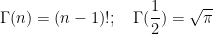
where

is the Gamma function. If we formally take Fourier transforms of this identity, we obtain
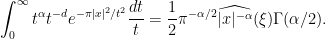
Another change of variables shows that

and so we conclude (formally) that

thus solving the problem of what the constant multiple of 
Exercise 35 Give a rigorous proof of (9) for
(when both sides are locally integrable) in the sense of distributions. (Hint: basically, one needs to test the entire formal argument against an arbitrary Schwartz function.) The identity (9) can in fact be continued meromorphically in
Specialising back to the current situation with 
we see that

and similarly

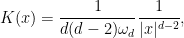
and so from (7) we see that one choice of the fundamental solution

leading to an explicit (and rigorously derived) solution

to the Poisson equation (6) in 
Exercise 36 Without using the theory of distributions, give an alternate (and still rigorous) proof that the function
Exercise 37
- Show that for any
where
is the volume of the unit ball in
- Show that for
.
- Show that for
, a fundamental solution is given by the locally integrable function
.
This we see that for the Poisson equation,
Similar methods can solve other constant coefficient linear PDE. We give some standard examples in the exercises below.
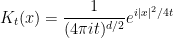
Exercise 38 Let
to the heat equation
with initial data
for some Schwartz function
for
is the heat kernel
(This solution is unique assuming certain smoothness and decay conditions at infinity, but we will not pursue this issue here.)

Exercise 39 Let
to the Schrödinger equation
with initial data
, where
and we use the standard branch of the complex logarithm (with cut on the negative real axis) to define
. (Hint: You may wish to investigate the Fourier transform of
, where
is a complex number with positive real part, and then let
to
follows in the heat kernel case by the theory of approximations to the identity, whereas the convergence in the Schrödinger case is much more subtle, and is best seen via Fourier analysis.)
Exercise 40 Let
to the wave equation
with initial data
for some Schwartz functions
for
where
is Lebesgue measure on the sphere
, and the derivative
is defined in the Newtonian sense
, with the limit taken in the sense of distributions.


Remark 5 The theory of (tempered) distributions is also highly effective for studying variable coefficient linear PDE, especially if the coefficients are fairly smooth, and particularly if one is primarily interested in the singularities of solutions to such PDE and how they propagate; here the Fourier transform must be augmented with more general transforms of this type, such as Fourier integral operators. A classic reference for this topic is the four volumes of Hörmander’s “The analysis of linear partial differential operators”. For nonlinear PDE, subspaces of the space of distributions, such as Sobolev spaces, tend to be more useful.

171 comments
Comments feed for this article
8 May, 2014 at 10:22 pm
Anonymous
Dear Dr. Tao,
In the process of solving Exercise 40, how do we define the in Fourier transform of a tempered distribution? For, example, let \lambda be a tempered distribution then (F\lambda) (f)=\lambda(Ff) or (F\lambda) (f)=\lambda(F^{-1}f), where F is denoting the Fourier transform?
9 May, 2014 at 7:25 am
Terence Tao
See equation (5).
9 May, 2014 at 8:09 pm
Anonymous
Dear Dr. Tao,
Are we supposed to use Kirchhoff’s formula to get the distribution K_{t} in Exercise 40?
Thanks
.
14 May, 2014 at 8:13 pm
Anonymous
Dear Dr. Tao,
In Exercise 40, what is the meaning of “Newtonian Sense” and how to use it in solving this Exercise?
Thanks!
14 May, 2014 at 8:28 pm
Terence Tao
http://en.wikipedia.org/wiki/Newton_quotient
14 May, 2014 at 10:47 pm
Anonymous
Just a minor comment for correction, in Exercise 40 isn’t it “… for some Schwartz functions {f} and {g} …” instead of “… for some Schwartz functions {f} is given by the formula …?”
[Corrected, thanks – T.]
20 August, 2015 at 5:04 am
KE operator and eigenfunctions
[…] I could explain what's going on but it will involve a long sojourn into distribution theory: https://terrytao.wordpress.com/2009/04/19/245c-notes-3-distributions/#more-2072 Really your teacher needs to explain it – post here with what he/she says – it should prove […]
26 August, 2015 at 6:52 am
Anonymous
In some books, a distribution on is defined as a linear functional
  with the following property
Suppose is a sequence in
  such that
There exists a compact subset of
of  such that
for all
and
as
Then as
as  .
.
Is it exactly the same as the distributions defined in this note?
[Yes; see Exercise 4(iii). -T.]
27 August, 2015 at 10:52 am
Anonymous
What is the weak derivative of the distribution defined in Exercise 12? It seems that p.v.(1/x^2) is not well defined…
27 August, 2015 at 11:17 am
Terence Tao
If one chases the definitions and integrates by parts, one has
So the derivative of p.v. 1/x is a renormalised principal value of -1/x^2.
27 August, 2015 at 12:10 pm
Anonymous
Hmm, how can one get the last line?
[Taylor expansion -T.]
28 August, 2015 at 7:21 am
Anonymous
It seems that this relates to https://en.wikipedia.org/wiki/Hadamard_regularization
But I don’t see why the limit exists…
28 August, 2015 at 7:35 am
Anonymous
Can one say that the limit in the last line exists since it is “equal” to , the existence of which has been proven in Ex. 12? It looks like a circular argument to me since in the very beginning one assumes the existence of
  .
.
[Yes, the existence of the earlier limits (which indeed follows from the easily verified fact that the distributional derivative of a distribution is again a distribution, together with Exercise 12) can be used to establish the existence of the later limits. It is also instructive to establish (again, using Taylor expansion) directly that the later limit is of a Cauchy sequence and thus convergent. -T.]
29 August, 2015 at 1:25 pm
Anonymous
I read somewhere before but I don’t remember exactly in what book:
Let $(a_n)$ be a strictly decreasing (I don’t remember if it is increasing or decreasing) positive sequence such that . If we defines
where , then
  converges (uniformly) to a function in
  .
.
Has anybody here seen a reference for such constructions of a nontrivial test function before? It seems that Exercise 1(i) is more standard.
18 September, 2015 at 1:25 pm
Anonymous
Stop cheating on math M541 homework.
2 November, 2015 at 7:06 pm
275A, Notes 4: The central limit theorem | What's new
[…] in the sense of distributions that arises in distribution theory (discussed for instance in this previous blog post), however strictly speaking the two notions of convergence are distinct and should not be confused […]
9 November, 2015 at 6:52 am
Anonymous
When construct an approximation to the identity, is there a particular reason that one chooses sequence instead of a continuous version
  ?
?
9 November, 2015 at 7:00 am
Anonymous
In Exercise 5(ii), does one need to assume that first in order to argue that “
 converges in
  to
to  “?
“?
9 November, 2015 at 10:25 am
Terence Tao
No, this is implicitly part of the conclusion (but this follows easily from Young’s inequality or Minkowski’s inequality).
If one only assumes local integrability or on
on  , then one needs compact support of the approximating sequence
  , as otherwise the tail of
  could interact with an arbitrarily large growth of
  and it is not even immediate that
  is anywhere finite, let alone convergent to anything interesting.
In most applications there is not much difference between using a discrete sequence of approximations rather than a continuous sequence, but using a countable discrete sequence makes it essentially trivial to establish measurability of any limit objects obtained, and also there are some sequential compactness results one can exploit when working with a discrete sequence that are not easily available in the continuous setting. (Of course in many situations one can use topological compactness as a substitute for sequential compactness, e.g. use topological Banach-Alaoglu in place of sequential Banach-Alaoglu.)
9 November, 2015 at 7:12 am
Anonymous
If is locally integrable or more generally
  , can one have the similar fact in Exercise 5?
9 November, 2015 at 11:55 am
Anonymous
In Exercise 1(iv), what is ? I’ve looked it up in your textbook and I didn’t find it there.
[See Exercise 1.10.7 (or Exercise 7 of 245B Notes 12), or also Exercise 1.10.17, Remark 1.10.16, etc..]
9 November, 2015 at 12:03 pm
Anonymous
In Exercise 9
if a sequence of locally integrable functions converge in to a limit…
What is the topology defined for ?
?
[The topology of is the topology generated by the seminorms
  for compact
  , as in Example 1.9.5. -T]
30 November, 2015 at 5:49 pm
Anonymous
Can one safely replace with any open set
  in this note to get the theory of distribution on
  ?
?
30 November, 2015 at 6:53 pm
Terence Tao
The theory of distributions localises fairly easily (basically just replace with
with  ). But the theory of tempered distributions is significantly more difficult to work with on domains, because it is not obvious how to define the Schwartz class on a domain (and because the main tool that makes the tempered distribution concept useful, namely the distributional Fourier transform, is not obviously available).
9 March, 2016 at 12:26 pm
Anonymous
I’m confused with the distributional derivatives in the setting of linear PDE. When one uses the formula
to define , is
, is  just the “formal adjoint” of
  ? For general
  , when one works in a boundary value problem in PDE (say Dirichlet problem or the Neumann problem for the Laplacian equations), should the adjoint
  depend also on the boundary conditions so that one has different definitions of the distributional derivative of the same differential operator ?
9 March, 2016 at 1:58 pm
Terence Tao
For distributions on a domain , the test functions
  involved are in
  , so they vanish to infinite order on the boundary. In particular, the precise notion of adjoint used is not relevant, as they will all agree on these test functions; in particular, the formal adjoint suffices. But one certainly has to take boundary issues into account when attempting to extend a distribution on
  to all of
  ; the situation here is more subtle than the corresponding situation with measurable functions, in which one can simply extend the function by zero outside of the domain. In general, the extension operation on distributions is not unique, which is related to the non-uniqueness of the adjoint operator when applied to more general functions than
  functions.
31 December, 2015 at 2:39 pm
Anonymous
Given a distribution , can we in general find a distribution
  with
with  as its distributional derivative?
[Yes; this is a good exercise for you to establish. The key point is that the test functions of mean zero form a hyperplane in the space of all test functions, in that any test function can be made mean zero by subtraction of a scalar multiple of a fixed reference test function. -T.]
11 May, 2016 at 4:48 pm
Anonymous2
A result due to de Rham says the following:
Let ,
,  , be distributions, where
  is a domain in
  . Then
  for some
  iff
iff  for all
  with
with  .
.
Does this contradicts the positive answer to the question above?
11 May, 2016 at 5:57 pm
Terence Tao
No; the previous question concerned only the one-dimensional case (or of a single partial derivative, rather than the full gradient), in which case the condition
  forces
  to vanish identically.
20 January, 2016 at 11:50 am
Anonymous
How do we see that ” embeds ‘continuously’ into
  ”
”
[Easiest way is via nets – show that every net that converges in also converges in the Schwartz topology. Or one can explicitly show that pullbacks of basic open sets are open. -T.]
17 February, 2016 at 5:01 pm
Debanjana Kundu
I was wondering if when we’re in and we know that
  , also
  ; for a test function
  if
if  is not in the support of
  can we say
  for all
  ?
?
10 March, 2016 at 3:09 am
Anonymous
i am in grade 7 and i knew about your iq
30 March, 2016 at 10:16 am
Anonymous
In Exercise 5(i), I get
and
But I don’t see how to go on. Do you have a hint?
30 March, 2016 at 10:37 am
Terence Tao
30 March, 2016 at 1:56 pm
jack
Instead of , one needs a bounded for
  , I think?
Consider the standard symmetric mollifier and
and  . Fix
. Fix  . For large enough
  ,
,  uniformly in
Why do we need "chop up the integral into two pieces"? Am I doing something wrong here?
30 March, 2016 at 2:10 pm
Terence Tao
Thanks for the correction. I had in mind a more general notion of approximation to the identity than the one that is in this post (in which some leakage of mass outside of a small ball is permitted), but you are right that with the notion of approximation to the identity used here, one does not need to decompose the integral.
4 April, 2016 at 3:56 pm
Anonymous
When one tries to upgrade the convergence to uniform convergence on , the proof above certainly would not work. But do you have a counterexample that one cannot upgrade the compact convergence? Why is compactness crucial here?
30 March, 2016 at 2:14 pm
Anonymous
What can one say in general for Exercise 5? Let for some function space
  such that
  makes sense. Can one always expect that
  in some convergence mode $latex $Y$ (or there are cases that not convergent in any mode at all)?
31 March, 2016 at 12:28 pm
Anonymous
In Exercise 5(ii), do you have a quick counterexample for ?
?
31 March, 2016 at 1:26 pm
Terence Tao
Uniform limits of continuous functions are necessarily continuous.
4 April, 2016 at 10:59 am
Anonymous
In Exercise 5(iii), what is the definition of when
when  is a vector value function? Perhaps you mean
 ?
?
4 April, 2016 at 1:15 pm
Terence Tao
Yes. By default, operations on scalar-valued functions are understood to act componentwise on vector-valued functions unless otherwise stated.
5 July, 2016 at 3:21 pm
Anonymous
Since embeds continuously into
  (with a dense image), we see that the space of tempered distributions can be embedded into the space of distributions.
How “good” is the embedding? In other words, is every tempered distribution locally integrable? Or is it in the “basic two examples of distributions”?
[No. For instance, the Dirac delta distribution is tempered, but not locally integrable. -T.]
30 August, 2016 at 6:33 am
Anonymous
In your definition of the “approximation to the identity”, is the third condition “whose supports shrink to the origin” equivalent to the following condition?
where the limit is understood in the space of Schwartz distributions.
22 September, 2016 at 9:53 pm
246A, Notes 1: Complex differentiation | What's new
[…] by the way, can be largely explained using the theory of distributions, as covered for instance in this previous post, but this is beyond the scope of the current […]
15 October, 2016 at 6:31 am
Anonymous
I don’t see in the notes if the following is true:
the weak derivative, if exists, must be unique.
I found that I end up with examining the following
if is locally integrable and
for all test functions , then
  a.e.
a.e.
I don’t find a proof here. Would you give me a hint that how this can be proved?
15 October, 2016 at 10:48 pm
Terence Tao
Use a limiting argument to show that if is orthogonal to all test functions, then it is also orthogonal to indicator functions of bounded measurable sets. Then argue by contradiction.
1 February, 2018 at 8:27 am
Anonymous
Would anyone elaborate the hint? (1)Where does this set of notes show that the set of test functions is dense in the set of indicator functions of bounded measurable sets? (2) What does the “contradiction” mentioned above refer to?
17 February, 2017 at 9:57 pm
254A, Notes 2: The central limit theorem | What's new
[…] in the sense of distributions that arises in distribution theory (discussed for instance in this previous blog post), however strictly speaking the two notions of convergence are distinct and should not be confused […]
2 August, 2017 at 5:42 am
LR
Dear Prof. Tao,
I suggest you to take a look at “Multiplication of the Distributions”, by Colombeau, which have some thoughts about applying it to nonlinear problems and the “Impossibility of multiplication” cited by Schwartz.
11 February, 2018 at 4:45 am
Sébastien
In your excellent PCM note on distributions, you mention that distributions can be composed both ways by suitably smooth functions. Was this a typo or not? Indeed, here and on the internet, I can only find composition in the “apply the true function first” order, and whenever people speak of the exponential of the Gaussian Free Field, they insist on the “one cannot a priori take the exponential of a distribution” issue, so I am confused now.
11 February, 2018 at 11:00 am
Terence Tao
Oops, that is indeed a typo. Distributions can be composed on the right with smooth functions but not on the left in general.
11 February, 2018 at 12:00 pm
Sébastien
Thank you very much!
19 March, 2018 at 8:49 am
Anonymous
Probably too late but I am curious. Would you define |delta(x)|=delta(x)?
I think there might be reasons for doing it but also reasons for not doing it.
19 March, 2018 at 6:26 pm
Terence Tao
Sure; one can for instance view this as a (somewhat degenerate) special case of the concept of a total variation of a measure. In general, though, it is only the measures of finite total variation for which one has a meaningful absolute value; more general distributions, such as the (distributional) derivative of
of  , do not have any particularly useful notion of an absolute value.
20 March, 2018 at 2:41 am
Anonymous
[sorry I am messing up with latex]
Thank you very much for your answer. What bothers me is that the reasoning used to explain why we do not define \delta^2 also might be invoked for |\delta|. If one takes the functions f_n(x)= n*c_n*\mbox{sinc}(n*x)/\mbox{rect}(x)
where c_n is an appropriate constant, then it seems to me that f_n\to \delta, but |f_n| does not converge. Am I missing something here?
20 March, 2018 at 7:42 am
Terence Tao
I do not know what the rect(x) function is, but it is certainly the case that the operation (as defined on “nice” functions) is not continuously extendible to the space of all distributions, much as is the case with
  . So there is no meaningful notion of the absolute value of an arbitrary distribution. However, if one restricts to the subclass of distributions that are measures of finite total variation, then
  becomes a continuous operation (using now the total variation topology), and so one can define
  for
for  in this class. (The sequence you provide will likely not converge in the total variation topology, but only in the distributional topology.)
20 March, 2018 at 3:12 pm
Anonymous
Thank you very much, I think I understand although I am a bit surprised by this idea of considering a subclass of measures of finite total variation. I wrote the functions in a wrong way but I meant to multiply n*sinc(n*x) by the indicator function of an interval say like [-1,1] and rescale appropriately to have integral =1. But actually even n*sinc(n*x) would have worked for my concern. ; if I consider again n*sinc(n*x) then this converges to
  in distribution and its square does converge to \delta too… so we might consider L_2 and define \delta^2?… mm…. ok I don’t want to bother further, you helped already enough, thank you very much again! :)
I thought (I am not a professional mathematician) one should usually require nice behaviour over any converging sequence in the distributional topology. I will think more about it.
– Actually, now I am puzzled by
28 April, 2018 at 5:55 pm
Anonymous
Since Wolff’s notes are used in 271A, I think my following question is related to this post.
In an estimate, the author gets (the appendix of Chapter 2 The Schwartz Space) a pointwise bound:


 instead of
  . It is said in Wolff’s notes that one can simply do it using rescaling. Can any one elaborate how the rescaling is done?
where
But what one really needs is the bound with
28 April, 2018 at 5:59 pm
Anonymous
The original goal is to prove by induction that
 where
where  .
.
with
The course should be MATH 247A: http://www.math.ucla.edu/~tao/247a.1.06f/
29 April, 2018 at 1:32 pm
Terence Tao
Apply the previous bound to the function .
.
29 April, 2018 at 1:50 pm
Anonymous
In the first comment, it should be that “But what one really needs is the bound with instead of
  .
.
I find that I messed up with the change of variables calculations. In the simplest case, one has
and hence
Thanks!
12 May, 2018 at 3:22 pm
Anonymous
Considering both Exercise 1 and 5, I still can’t see how to answer the question in https://terrytao.wordpress.com/2009/04/06/the-fourier-transform/#comment-498013
If one uses an approximation to the identity, , then

 and
and  for
for  . This seems to be quite close to what I want. But there is no guarantee that

in both
On the other hand, since , there exists
  so that
  . So one can approximate
  by
by

 .
.
where
Since as well, similarly one has

 But then one has two different sequences, $\phi_n*h and \phi_n*g$.
where
12 May, 2018 at 3:32 pm
Anonymous
In the first case, I have already had
in both the
where
But it is known that . If one can control the decay (and retain the differentiability) of
  to get
  , then the proof would be complete…
13 May, 2018 at 7:45 am
Terence Tao
In addition to convolving with a mollifier, one should also multiply by a smooth cutoff such as to obtain compact support (which, together with the smoothness provided by the mollifier, place one in the Schwartz class without difficulty).
5 July, 2018 at 8:39 pm
Josh Chen
Is there any reference or literature you might point to for generalized functions/distributions/Schwartz functions in infinite dimensions? It’s interesting to consider tempered distributions rather than for example Gaussian measures for PDEs with random coefficient fields or time stochastic PDE processes..
13 August, 2018 at 3:24 am
Daniel Pires
Hi professor Tao! I was trying to solve this one problem and I thought it was related to this notes than
than
if
(here denotes the inverse Fourier Transform).
Do you have any hint for how can I solve this?
13 August, 2018 at 7:33 am
Terence Tao
Basically one needs some decay estimates on the Fourier transform (it turns out in this case that it decays like ). One can see this for instance by dyadic decomposition (splitting
  into a bunch of rescaled bump functions). In this particular case there may also be some exact formulae that could be helpful (there are some computations of related kernels for instance in Stein’s “singular integrals”, possibly also in Stein-Weiss’s “Fourier analysis on Euclidean spaces”).
3 September, 2018 at 3:13 pm
254A, Notes 0: Physical derivation of the incompressible Euler and Navier-Stokes equations | What's new
[…] but we will adopt the viewpoint of the theory of distributions (as reviewed for instance in these old lecture notes of mine) and consider approximation against test functions in spacetime, thus we assume […]
2 October, 2018 at 3:47 pm
254A, Notes 2: Weak solutions of the Navier-Stokes equations | What's new
[…] some key aspects of the theory. A more comprehensive discussion of distributions may be found in this previous blog post. To avoid some minor subtleties involving complex conjugation that are not relevant for this post, […]
26 October, 2018 at 12:21 am
Rajnikant Snha
Dear Professor Tao,
On p 172, line number 5, Rudin’s Functional Analysis, there is a limit in the space of test functions. It seems to me wrong. Can you supply its intelligible proof.
With thanks in advance.
28 November, 2018 at 1:58 pm
254A, Notes 3: Local well-posedness for the Euler equations | What's new
[…] some key aspects of the theory. A more comprehensive discussion of distributions may be found in this previous blog post. To avoid some minor subtleties involving complex conjugation that are not relevant for this post, […]
7 February, 2019 at 7:14 am
Laszlo
Does the convolution algebra of compactly supported distributions on $R^n$ have any delicate algebraic properties (like Noether ring, etc.)?
7 February, 2019 at 8:34 am
Terence Tao
I did a bit of poking around and found this recent paper by Vogt on the subject: https://mathscinet.ams.org/mathscinet-getitem?mr=3858282 . Presumably the references cited in the introduction will describe the current state of knowledge in this direction.
7 February, 2019 at 11:11 am
Laszlo
Thx!
28 June, 2019 at 4:57 pm
acx01bc
You should mention![\delta(t) = \lim_{n \to \infty} n 1_{t \in [0,1/n]}](https://s0.wp.com/latex.php?latex=%5Cdelta%28t%29+%3D+%5Clim_%7Bn+%5Cto+%5Cinfty%7D+n+1_%7Bt+%5Cin+%5B0%2C1%2Fn%5D%7D&bg=ffffff&fg=545454&s=0&c=20201002) which works everywhere even for things such as
which works everywhere even for things such as  , the only point is that the limit doesn’t need to converge in the sense of distributions.
29 August, 2019 at 9:34 am
Victor
Dear Professor Tao, I am trying to prove the following statement:
Let be the space of the distributions with compact support. Suppose that
  in
in  (In the sense
  for all
  .Then, there exist a compact
  such that
  for all
  .
.
Is there an easy way to prove it?
30 August, 2019 at 7:56 am
Terence Tao
Perhaps I am misreading your question, but it appears that “moving bump” type examples such as![u_n = 1_{[n,n+1]}](https://s0.wp.com/latex.php?latex=u_n+%3D+1_%7B%5Bn%2Cn%2B1%5D%7D&bg=ffffff&fg=545454&s=0&c=20201002) or “spreading bump” examples such as
or “spreading bump” examples such as ![u_n = \frac{1}{n} 1_{[0,n]}](https://s0.wp.com/latex.php?latex=u_n+%3D+%5Cfrac%7B1%7D%7Bn%7D+1_%7B%5B0%2Cn%5D%7D&bg=ffffff&fg=545454&s=0&c=20201002) would give counterexamples to your claim.
would give counterexamples to your claim.
6 May, 2024 at 12:09 pm
Anonymous
I think these examples don’t work, since we can construct a smooth function $varphi$ such that $langle u_n, vaprhi rightarrow infty.$
6 November, 2019 at 4:35 pm
254A, Supplement 2: A little bit of complex and Fourier analysis | What's new
[…] exercise is intended for readers familiar with distribution theory, as discussed for instance in this previous blog post.) If is holomorphic on an open set , establish the […]
8 April, 2020 at 11:13 am
Tingzhou
Hi Prof. Tao
Can you give more hints about Exercise 37: “This we see that for the Poisson equation, {d=2} is a “critical” dimension, requiring a logarithmic correction to the usual formula?” How can we get the “logarithmic correction” to the Fourier transform of
8 April, 2020 at 12:40 pm
Terence Tao
The logarithmic correction basically arises from the need to add a correction term (in the spirit of Exercise 13) to interpret as a distribution as it is no longer absolutely integrable in dimensions
  .
.
29 October, 2020 at 12:15 pm
Anonymous
(Indeed, by Exercise 46 of Notes 2, it is not possible to find a non-trivial test function whose Fourier transform is again a test function.)
There is no Exercise 46 in Notes 2. Typo?
[Corrected, thanks – T.]
29 December, 2022 at 9:13 am
Anonymous
In, Exercise 1(iii) ( Urysohn lemma), let
  be the test function in 1(i). By scaling, one can define
  to control the size of its support.
By the Urysohn lemma, one can find such that it equals
  in the compact set
  and
and  in the complement of a compact set
  where
where  . To get the desired
  function, take
  where
where  is chosen so that the (compact) support
  of
of  is contained in
  .
.
How can one construct so that taking convolution should not “contaminate” the value
  of the function
  on
on  ?
?
31 December, 2022 at 7:10 pm
Terence Tao
Choose to equal
  on a slightly larger region than
  . I’m not aware of a completely soft argument to construct the smooth cutoff function without using an explicit device such as convolution.
29 December, 2022 at 9:16 am
Anonymous
Is some sort of “existence argument” rather than explicit construction proof possible for Exercise 1(iii)?
30 December, 2022 at 2:30 pm
Anonymous
… or equivalently, the ball
Could you elaborate on how this is equivalent to continuity of the seminorm ? By homogeneity, the condition above implies that the ball
  is open in
  for every positive constant
  . How does one show that
  is also open?
31 December, 2022 at 7:48 pm
Terence Tao
By the triangle inequality, is the union of open balls in the
  seminorm.
30 December, 2022 at 3:05 pm
Anonymous
In Exercise 2, one direction follows directly from the definition of “good” seminorms:
Suppose for some compact , which contains the supports of
  and
and  , one has
  converges to
  in the smooth topology of
  . If
. If  is a good seminorm on
  , then by continuity, one has
  .
.
How does one show the other direction? If converges to
  in the topology of
  , equivalently, in every good seminorm
  , how can one identify the compact
  that contains all the supports of
  and
and  ?
?
[Argue by contradiction – T.]