
A recurring theme in mathematics is that of duality: a mathematical object 
- Vector space duality A vector space
over a field
can be described either by the set of vectors inside
from
). (If one is working in the category of topological vector spaces, one would work instead with continuous linear functionals; and so forth.) A fundamental connection between the two is given by the Hahn-Banach theorem (and its relatives).
- Vector subspace duality In a similar spirit, a subspace
of
. Again, the Hahn-Banach theorem provides a fundamental connection between the two perspectives.
- Convex duality More generally, a (closed, bounded) convex body
in a vector space
- Ideal-variety duality In a slightly different direction, an algebraic variety
can be viewed either “in physical space” or “internally” as a collection of points in
- Hilbert space duality An element
in a Hilbert space
can either be thought of in physical space as a vector in that space, or in momentum space as a covector
on that space. The fundamental connection between the two is given by the Riesz representation theorem for Hilbert spaces.
- Semantic-syntactic duality Much more generally still, a mathematical theory can either be described internally or syntactically via its axioms and theorems, or externally or semantically via its models. The fundamental connection between the two perspectives is given by the Gödel completeness theorem.
- Intrinsic-extrinsic duality A (Riemannian) manifold
can either be viewed intrinsically (using only concepts that do not require an ambient space, such as the Levi-Civita connection), or extrinsically, for instance as the level set of some defining function in an ambient space. Some important connections between the two perspectives includes the Nash embedding theorem and the theorema egregium.
- Group duality A group
can be described either via presentations (lists of generators, together with relations between them) or representations (realisations of that group in some more concrete group of transformations). A fundamental connection between the two is Cayley’s theorem. Unfortunately, in general it is difficult to build upon this connection (except in special cases, such as the abelian case), and one cannot always pass effortlessly from one perspective to the other.
- Pontryagin group duality A (locally compact Hausdorff) abelian group
, or by listing the characters
(i.e. continuous homomorphisms from
). The connection between the two is the focus of abstract harmonic analysis.
- Pontryagin subgroup duality A subgroup
. One of the fundamental connections between the two is the Poisson summation formula.
- Fourier duality A (sufficiently nice) function
on a locally compact abelian group
) can either be described in physical space (by its values
at each element
of
at elements
of the Pontryagin dual
- The uncertainty principle The behaviour of a function
at physical scales above (resp. below) a certain scale
is almost completely controlled by the behaviour of its Fourier transform
at frequency scales below (resp. above) the dual scale
and vice versa, thanks to various mathematical manifestations of the uncertainty principle. (The Poisson summation formula can also be viewed as a variant of this principle, using subgroups instead of scales.)
- Stone/Gelfand duality A (locally compact Hausdorff) topological space
algebra
of continuous complex-valued functions on that space, or (in the case when
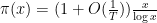
I have discussed a fair number of these examples in previous blog posts (indeed, most of the links above are to my own blog). In this post, I would like to discuss the uncertainty principle, that describes the dual relationship between physical space and frequency space. There are various concrete formalisations of this principle, most famously the Heisenberg uncertainty principle and the Hardy uncertainty principle – but in many situations, it is the heuristic formulation of the principle that is more useful and insightful than any particular rigorous theorem that attempts to capture that principle. Unfortunately, it is a bit tricky to formulate this heuristic in a succinct way that covers all the various applications of that principle; the Heisenberg inequality 
- A function which is band-limited (restricted to low frequencies) is featureless and smooth at fine scales, but can be oscillatory (i.e. containing plenty of cancellation) at coarse scales. Conversely, a function which is smooth at fine scales will be almost entirely restricted to low frequencies.
- A function which is restricted to high frequencies is oscillatory at fine scales, but is negligible at coarse scales. Conversely, a function which is oscillatory at fine scales will be almost entirely restricted to high frequencies.
- Projecting a function to low frequencies corresponds to averaging out (or spreading out) that function at fine scales, leaving only the coarse scale behaviour.
- Projecting a frequency to high frequencies corresponds to removing the averaged coarse scale behaviour, leaving only the fine scale oscillation.
- The number of degrees of freedom of a function is bounded by the product of its spatial uncertainty and its frequency uncertainty (or more generally, by the volume of the phase space uncertainty). In particular, there are not enough degrees of freedom for a non-trivial function to be simulatenously localised to both very fine scales and very low frequencies.
- To control the coarse scale (or global) averaged behaviour of a function, one essentially only needs to know the low frequency components of the function (and vice versa).
- To control the fine scale (or local) oscillation of a function, one only needs to know the high frequency components of the function (and vice versa).
- Localising a function to a region of physical space will cause its Fourier transform (or inverse Fourier transform) to resemble a plane wave on every dual region of frequency space.
- Averaging a function along certain spatial directions or at certain scales will cause the Fourier transform to become localised to the dual directions and scales. The smoother the averaging, the sharper the localisation.
- The smoother a function is, the more rapidly decreasing its Fourier transform (or inverse Fourier transform) is (and vice versa).
- If a function is smooth or almost constant in certain directions or at certain scales, then its Fourier transform (or inverse Fourier transform) will decay away from the dual directions or beyond the dual scales.
- If a function has a singularity spanning certain directions or certain scales, then its Fourier transform (or inverse Fourier transform) will decay slowly along the dual directions or within the dual scales.
- Localisation operations in position approximately commute with localisation operations in frequency so long as the product of the spatial uncertainty and the frequency uncertainty is significantly larger than one.
- In the high frequency (or large scale) limit, position and frequency asymptotically behave like a pair of classical observables, and partial differential equations asymptotically behave like classical ordinary differential equations. At lower frequencies (or finer scales), the former becomes a “quantum mechanical perturbation” of the latter, with the strength of the quantum effects increasing as one moves to increasingly lower frequencies and finer spatial scales.
- Etc., etc.
- Almost all of the above statements generalise to other locally compact abelian groups than
or
, in which the concept of a direction or scale is replaced by that of a subgroup or an approximate subgroup. (In particular, as we will see below, the Poisson summation formula can be viewed as another manifestation of the uncertainty principle.)
I think of all of the above (closely related) assertions as being instances of “the uncertainty principle”, but it seems difficult to combine them all into a single unified assertion, even at the heuristic level; they seem to be better arranged as a cloud of tightly interconnected assertions, each of which is reinforced by several of the others. The famous inequality
The uncertainty principle (as interpreted in the above broad sense) is one of the most fundamental principles in harmonic analysis (and more specifically, to the subfield of time-frequency analysis), second only to the Fourier inversion formula (and more generally, Plancherel’s theorem) in importance; understanding this principle is a key piece of intuition in the subject that one has to internalise before one can really get to grips with this subject (and also with closely related subjects, such as semi-classical analysis and microlocal analysis). Like many fundamental results in mathematics, the principle is not actually that difficult to understand, once one sees how it works; and when one needs to use it rigorously, it is usually not too difficult to improvise a suitable formalisation of the principle for the occasion. But, given how vague this principle is, it is difficult to present this principle in a traditional “theorem-proof-remark” manner. Even in the more informal format of a blog post, I was surprised by how challenging it was to describe my own understanding of this piece of mathematics in a linear fashion, despite (or perhaps because of) it being one of the most central and basic conceptual tools in my own personal mathematical toolbox. In the end, I chose to give below a cloud of interrelated discussions about this principle rather than a linear development of the theory, as this seemed to more closely align with the nature of this principle.
— 1. An informal foundation for the uncertainty principle —
Many of the manifestations of the uncertainty principle can be heuristically derived from the following informal heuristic:
Heuristic 1 (Phase heuristic) If the phase
of a complex exponential
fluctuates by less than
for
(e.g. a convex set, or more generally an approximate subgroup), then the phase
For instance, according to this heuristic, on an interval ![{[-R,R]}](https://s0.wp.com/latex.php?latex=%7B%5B-R%2CR%5D%7D&bg=ffffff&fg=000000&s=0&c=20201002)


We remark in passing that, the above heuristic can also be viewed as the informal foundation for the principle of stationary phase. This is not coincidental, but will not be the focus of the discussion here.
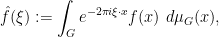
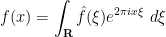
Let’s give a few examples to illustrate how this heuristic informally implies some versions of the uncertainty principle. Suppose for instance that a function 

(Other normalisations of the Fourier transform are possible, but this does not significantly affect the discussion here.) We assume that the function is nice enough (e.g. absolutely integrable will certainly suffice) that one can define the Fourier transform without difficulty.
If 
![{x \in [-R,R]}](https://s0.wp.com/latex.php?latex=%7Bx+%5Cin+%5B-R%2CR%5D%7D&bg=ffffff&fg=000000&s=0&c=20201002)


A similar heuristic calculation using the Fourier inversion formula

shows that if the Fourier transform ![{[-N, N]}](https://s0.wp.com/latex.php?latex=%7B%5B-N%2C+N%5D%7D&bg=ffffff&fg=000000&s=0&c=20201002)

![{[\xi_0-N, \xi_0+N]}](https://s0.wp.com/latex.php?latex=%7B%5B%5Cxi_0-N%2C+%5Cxi_0%2BN%5D%7D&bg=ffffff&fg=000000&s=0&c=20201002)


The same type of heuristic computation can be carried through in higher dimensions. For instance, if a function 


of
An important special case where the above heuristics are in fact exactly rigorous is when one does not work with approximate subgroups such as intervals
where 


wheere 

For instance, a measure 
Remark 1 Of course, in Euclidean domains such as
of formal Laurent series in a variable
over a finite field
One can view an interval such as ![{[-1/R,1/R]}](https://s0.wp.com/latex.php?latex=%7B%5B-1%2FR%2C1%2FR%5D%7D&bg=ffffff&fg=000000&s=0&c=20201002)


and when specialised to subspaces

We saw above that a function 
we note that if 
The above heuristic computations can be made rigorous in a number of ways. One basic method is to exploit the fundamental fact that the Fourier transform intertwines multiplication and convolution, thus

and

and similarly for the inverse Fourier transform. (Here, the convolution 
![{[-N,N]}](https://s0.wp.com/latex.php?latex=%7B%5B-N%2CN%5D%7D&bg=ffffff&fg=000000&s=0&c=20201002)

where 

![{[-1,1]}](https://s0.wp.com/latex.php?latex=%7B%5B-1%2C1%5D%7D&bg=ffffff&fg=000000&s=0&c=20201002)
Inverting the Fourier transform, we obtain the reproducing formula

where 


If one chose 


Another basic method to formalise the above heuristics, particularly with regard to “oscillation causes cancellation”, is to use integration by parts; this is discussed at this Tricki article.
— 2. Projections —
The restriction ![{1_{[-N,N]}(X) f := f 1_{[-N,N]}}](https://s0.wp.com/latex.php?latex=%7B1_%7B%5B-N%2CN%5D%7D%28X%29+f+%3A%3D+f+1_%7B%5B-N%2CN%5D%7D%7D&bg=ffffff&fg=000000&s=0&c=20201002)

![{1_{[-N,N]}(D) f}](https://s0.wp.com/latex.php?latex=%7B1_%7B%5B-N%2CN%5D%7D%28D%29+f%7D&bg=ffffff&fg=000000&s=0&c=20201002)
![\displaystyle \widehat{1_{[-N,N]}(D) f} := \hat f 1_{[-N,N]}](https://s0.wp.com/latex.php?latex=%5Cdisplaystyle++%5Cwidehat%7B1_%7B%5B-N%2CN%5D%7D%28D%29+f%7D+%3A%3D+%5Chat+f+1_%7B%5B-N%2CN%5D%7D&bg=ffffff&fg=000000&s=0&c=20201002)
is the orthogonal projection of ![{1_{[-N,N]}}](https://s0.wp.com/latex.php?latex=%7B1_%7B%5B-N%2CN%5D%7D%7D&bg=ffffff&fg=000000&s=0&c=20201002)
One can view the restriction operator ![{1_{[-N,N]}(X)}](https://s0.wp.com/latex.php?latex=%7B1_%7B%5B-N%2CN%5D%7D%28X%29%7D&bg=ffffff&fg=000000&s=0&c=20201002)

![{1_{[-N,N]}(D)}](https://s0.wp.com/latex.php?latex=%7B1_%7B%5B-N%2CN%5D%7D%28D%29%7D&bg=ffffff&fg=000000&s=0&c=20201002)
As before, one can work with other sets than intervals here. For instance, restricting a function 


More generally, one has

for any 
on one hand, and the forward Fourier transform formula

on the other.
The duality 


for some Hermitian (and time-independent) spatial operator 

then the solution to (2) is formally given by the formula

We thus see that the coefficients 


As a consequence, the heuristics of the uncertainty principle carry through here. Just as the behaviour of a function 


for any test function 


A similar analysis also holds for the solution operator

for the wave equation

on an arbitrary spatial Riemannian manifold 


From the finite speed of propagation property of the wave equation (which has been normalised so that the speed of light 


Another important uncertainty principle duality relationship is that between the (imaginary parts of the) zeroes 


and using rigorous versions of the heuristic factorisation

one can soon derive explicit formulae connecting zeroes and primes, such as

(see e.g. this blog post of mine for more discussion). Using such formulae, one can relate the zeroes of the zeta function in the strip 


— 3. Phase space and the semi-classical limit —
The above heuristic description of Fourier projections such as ![{1_{[-N,N]}(x)}](https://s0.wp.com/latex.php?latex=%7B1_%7B%5B-N%2CN%5D%7D%28x%29%7D&bg=ffffff&fg=000000&s=0&c=20201002)


Heuristically, 


Thus we conclude that the phase space region 
More generally, the number of degrees of freedom contained in a large region 

where 
![{1_{[-\infty,E]}(H)}](https://s0.wp.com/latex.php?latex=%7B1_%7B%5B-%5Cinfty%2CE%5D%7D%28H%29%7D&bg=ffffff&fg=000000&s=0&c=20201002)


The correspondence principle in quantum mechanics asserts that in the limit 

with a potential 

where 


where 


We now indicate (heuristically, at least) how (4) converges to (5) as 


where 


Before we analyse the equation (4), we first look at some simpler equations. First, we look at

where
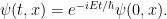
This phase rotation does not change the location

Next, we look at the transport equation

where 

the position

Combining the two, we see that an equation of the form

would also transport the position 

where 
this phase modulation does not change the position

Finally, we combine all these equations together, looking at the combined equation

Heuristically at least, the position

We remark that one can make the above quite rigorous by using the metaplectic representation.
This analysis was for 
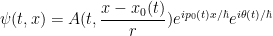
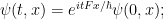
Now we return to the Schrödinger equation (4). If 

Similarly, if 


These Taylor expansions become increasingly accurate in the limit

where 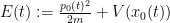
More generally, a Schrödinger equation

where 


and (6) leads us to the Hamilton equations of motion

It turns out that these heuristic computations can be made completely rigorous in the semi-classical limit

27 comments
Comments feed for this article
26 June, 2010 at 8:50 am
David
At the end of the discussion of zeta, should be
  .
.
[Corrected, thanks. – T.]
26 June, 2010 at 8:52 am
David
Also, the in the exponential is surpuflous. Sorry for the double comment!
[Corrected, thanks. – T.]
27 June, 2010 at 8:30 am
mfrasca
Hi Terry,
As you know, a duality principle holds true also in perturbation theory:
http://pra.aps.org/abstract/PRA/v58/i5/p3439_1
For a given problem with a small perturbation you can generally get a solution to the same one having the perturbation going to infinity.
Regards,
Marco
27 June, 2010 at 12:36 pm
Anonymous
There is a t missing in exponent of e^(-iE/h) in the equation just under “Then the evolution of this equation is given by a simple phase rotation: ”
[Corrected, thanks – T.]
28 June, 2010 at 11:31 am
Researcher
Great post! May I humbly suggest using a new tag “heuristics” for the posts like that? And anyway I’d be thrilled to see more posts on various heuristics in mathematics on your blog, with or without this tag :)
5 July, 2010 at 12:44 am
dmitin
http://en.wikipedia.org/wiki/Duality_(projective_geometry)
http://en.wikipedia.org/wiki/Duality_(projective_geometry)#Combinatorial_duality
11 August, 2010 at 8:30 pm
Anonymous
Professor Tao:
If we consider 1, 10 , 100, 1000… as basis we have a representation of integers in terms of these basis. I was wondering if there is a notion of harmonic analysis on integers apart from the fourier transform so that multiplication (which is just convolution with carry) could have a dual basis interpretation. Something like multiplication of polynomials using fft. It seems that the ordinary notion of Parseval’s theorem will not hold (or else product of sum of squares of digits of two numbers to be multiplied would be the sum of squares of the digits of the resulting integers which is untrue).
Thank you
18 August, 2010 at 5:57 am
Paul Shearer
Hi Terry,
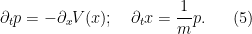
Another beautiful example of duality comes from optimization theory, in the form of the Fenchel dual to a function. The Fenchel dual has the following physical interpretation, which nicely illustrates your theme of “dual intrinsic/extrinsic” descriptions of an object:
“A particle in a convex potential well can be pushed to any desired equilibrium point x by applying an appropriate force p. There is a bijective map relating x and p: the forward map is
  , while the inverse is
  , where
  is the Fenchel dual to
  .”
.”
To be more formal, given a nice convex function , we can interpret it as a potential function that a particle rolls around in.
Let denote the inner product. Then the Fenchel dual to F is defined as
Let x be the point where the max is achieved. The point x can be interpreted as the equilibrium position of a particle in potential F when this particle is subjected to a constant “applied force” p. The function
can be interpreted as an effective potential induced by the applied force, and the Fenchel dual is implicitly finding x, the equilibrium point where this potential is minimized. With a little calc and algebra we find
(The negative is taken simply because the duality is cleaner if is convex rather than concave.) A little calculus shows that
(*)
completing the justification of the physical interpretation at the top of this post.
The derivation of this fact is intriguing in itself; by applying the multivariate chain rule to differentiate
with respect to p, we find
The fact is known from above, and arises from the fact that the particle is at equilibrium; thus the only change in the effective potential arises from the change in the “applied potential” with respect to p alone, holding x constant.
Another interesting fact: a nonrigorous but intuitively appealing derivation of the Fenchel dual, in particular the involutive property, is possible by the following geometric procedure:
1. draw a contour plot of some nice F.
2. draw a vector from 0 to a given equilibrium point x.
3. draw the applied force p as a vector pointing from point x to x + p.
Note that the two vectors drawn are now two sides of a parallelogram; the Fenchel dual is a function for which one can follow the exact same steps (1)-(3) again, but one uses the other two sides of the parallelogram and reverses the roles of p and x. After drawing this diagram, the involutive property of Fenchel duality becomes immediately obvious: taking the dual just means “flipping” the parallelogram over! :)
18 August, 2010 at 11:51 am
Paul Shearer
whoops! it’s supposed to be . sorry. Although I guess it’s still an interesting and nontrivial statement for n = 1. Just not as geometrically cool…
30 January, 2011 at 9:07 pm
Chen-bo Zhu
Hi Prof. Tao,
Before Remark 1, there is a typo: if H is a measure zero subgroup of H (which should be G). Also I think the statement that f^ is constant along cosets of the orthogonal complement may need a small revision since f can be a transversal derivative of a measure on H. [Corrected, thanks – T.]
Not sure if the following paragraph is appropriate as a follow-up to your blog, and so please feel free to remove this paragraph if it is not so.
There is a certain rigidity phenomenon of distributions with strong support properties, which may be considered as an another instance of the uncertainty principle:
Click to access rigidity-distribution.pdf
Regards, Chen-bo
30 March, 2011 at 9:33 am
Higher order Fourier analysis « What’s new
[…] was based primarily on my graduate course in the topic, though it also contains material from some additional posts related to linear and higher order Fourier analysis on the blog. It is available […]
4 August, 2011 at 6:53 pm
Localisation and compactness properties of the Navier-Stokes global regularity problem « What’s new
[…] the uncertainty principle (discussed in this post) suggests that . Finally, the linear term and nonlinear term have heuristic magnitudes about and […]
1 January, 2012 at 11:46 am
Montgomery’s uncertainty principle « What’s new
[…] One of the most fundamental principles in Fourier analysis is the uncertainty principle. It does not have a single canonical formulation, but one typical informal description of the principle is that if a function is restricted to a narrow region of physical space, then its Fourier transform must be necessarily “smeared out” over a broad region of frequency space. Some versions of the uncertainty principle are discussed in this previous blog post. […]
23 May, 2012 at 6:06 pm
Quora
What is an intuitive way of explaining how the “Fourier transform” works?…
Fourier transform is way of writing functions on a space as a superposition of symmetric functions. Depending on the space we are interested, there can be several symmetries associated to the function. For instance, the fourier transform on real line i…
17 July, 2015 at 4:01 pm
Lemme tell y’all about icosian calculus. | between bourbaki and me
[…] Sitting in a coffee shop, I wandered over to the wiki for the presentation of a group. A presentation is a natural idea in group theory, a compact way of describing a group by referring to a set of generators and relations between those generators. Fun fact, the presentation of a group is an example of an internal object description. This is part of a larger phenomenon in mathematics where we describe an object based on functions from similar objects into your object. For instance, the presentation is equivalent to a description of a map from a free group on a set of generators S into your group G. You essentially describe how to fold the free group up into your group! The internal description is in contrast with external, where you send maps out of your objects. In group theory, this is called representation theory. Tons more mind-blowing examples of internal-external definitions at Terry Tao’s blog. […]
10 December, 2015 at 12:13 pm
Decoupling and the Bourgain-Demeter-Guth proof of the Vinogradov main conjecture | What's new
[…] of Theorem 5.6 of Bourgain-Demeter-Guth, or my general discussion on the uncertainty principle in this previous blog post). This implies that , when restricted to , is essentially constant on “plates”, defined […]
14 March, 2017 at 9:17 am
On “external” definitions for computation | Windows On Theory
[…] to me to be an instance of moving to an external, as opposed to internal definition, in the sense described by Tao. (Please correct me if I’m wrong!) As Arkani-Hamed describes, a hugely important paper […]
5 January, 2020 at 11:58 pm
To lift and breathe – Tea and Skulls
[…] Internal descriptions stand in contrast with external descriptions. Can you guess what an external description might be like? If internal descriptions were maps into the group, then it would make sense if external descriptions were maps out of the group. Fortunately, things do make sense, and I’m not lying to you, so that’s exactly what external descriptions are. In group theory, the description of a group is called a representation. The study of representation is called representation. (If this internal-external business sounds cool to you, check out this dope post by Terry Tao: blog). […]
21 January, 2020 at 3:32 am
On generating functions in additive number theory, II: Lower-order terms and applications to PDEs | George Shakan
[…] By uncertainty principle heuristics, we expect , as defined in (1), to be constant on scales […]
5 March, 2020 at 7:14 pm
Daniel D
In (3) we have and then another expression that appears is
  , as I understand just a position and momentum satisfy heisenberg uncertainty, time and energy also do
  could
could  make sense?, thanks
6 March, 2020 at 8:18 am
Terence Tao
Well, it’s rather than
  . So if one splits
  then the more accurate form of the uncertainty principle heuristic regarding the primes should be
  . Thus, for instance, if one wants to count the number of primes in an interval of the form
 ![[x, x+x/T]](https://s0.wp.com/latex.php?latex=%5Bx%2C+x%2Bx%2FT%5D&bg=ffffff&fg=545454&s=0&c=20201002) (so that
(so that  is confined to an interval of length
  ), one should expect to need to control the Riemann zeta function
  for heights
  . And this is indeed the case if one looks at what the truncated Perron formula actually gives (see e.g., Proposition 12 of https://terrytao.wordpress.com/2014/12/09/254a-notes-2-complex-analytic-multiplicative-number-theory/ ).
2 July, 2020 at 7:16 pm
trucupey
Hi, professor Tao, maybe I am not understanding well but in the example 14 of what you called heuristically statements, shouldn’t it say “In the low frequency (or large scale) limit, position and frequency asymptotically behave like a pair of classical observables … ” instead of “In the high frequency (or large scale) limit, position and frequency asymptotically behave like a pair of classical observables …” ?
7 July, 2020 at 5:31 pm
Terence Tao
To achieve the semiclassical limit one has to make the product much larger than Planck’s constant
  . There are two ways to do this: either go to high frequencies (so that
  becomes large) or large scales (so that
  becomes large).
30 October, 2021 at 12:39 am
[scala] 프로그래밍에서 "대수"는 무엇을 의미합니까? - 리뷰나라
[…] 이중 공간 을 보는 이유 는 일반적으로 그 공간에서 생각하기가 더 쉽기 때문입니다. 예를 들어, 법선 벡터에 대해 법선 평면보다 생각하기가 더 쉬운 경우가 있지만 벡터로 평면 (하이 평면 포함)을 제어 할 수 있습니다 (이제 광선 추적기와 같이 익숙한 기하학적 벡터에 대해 말하고 있습니다). . […]
15 September, 2022 at 9:17 am
Adversarial examples and quant quakes – Research Notebook
[…] in the data by diffusely spreading out across a large number of predictors. There’s a generalized uncertainty principle at work a la Donoho and Stark […]
7 March, 2023 at 4:33 pm
Anonymous
Dr Tao: You mentioned that the Poisson summation formula can be interpreted as a variant of the uncertainty principle using “adelic” topology. I don’t know anything about adelic topology. Could you explain a bit more about the interpretation? Thanks.