Szemeredi’s proof of Szemeredi’s theorem

Szemerédi’s theorem asserts that all subsets of the natural numbers of positive density contain arbitrarily long arithmetic progressions.  Roth’s theorem is the special case when one considers arithmetic progressions of length three.  Both theorems have many important proofs using tools from additive combinatorics, (higher order) Fourier analysis, (hyper) graph regularity theory, and ergodic theory.  However, the original proof by Endre Szemerédi, while extremely intricate, was purely combinatorial (and in particular “elementary”) and almost entirely self-contained, except for an invocation of the van der Waerden theorem.  It is also notable for introducing a prototype of what is now known as the Szemerédi regularity lemma.

Back in 2005, I rewrote Szemerédi’s original proof in order to understand it better, however my rewrite ended up being about the same length as the original argument and was probably only usable to myself.  In 2012, after Szemerédi was awarded the Abel prize, I revisited this argument with the intention to try to write up a more readable version of the proof, but ended up just presenting some ingredients of the argument in a blog post, rather than try to rewrite the whole thing.  In that post, I suspected that the cleanest way to write up the argument would be through the language of nonstandard analysis (perhaps in an iterated hyperextension that could handle various hierarchies of infinitesimals), but was unable to actually achieve any substantial simplifications by passing to the nonstandard world.

A few weeks ago, I participated in a week-long workshop at the American Institute of Mathematics on “Nonstandard methods in combinatorial number theory”, and spent some time in a working group with Shabnam Akhtari, Irfam Alam, Renling Jin, Steven Leth, Karl Mahlburg, Paul Potgieter, and Henry Towsner to try to obtain a manageable nonstandard version of Szemerédi’s original proof.  We didn’t end up being able to do so – in fact there are now signs that perhaps nonstandard analysis is not the optimal framework in which to place this argument – but we did at least clarify the existing standard argument, to the point that I was able to go back to my original rewrite of the proof and present it in a more civilised form, which I am now uploading here as an unpublished preprint.   There are now a number of simplifications to the proof.  Firstly, one no longer needs the full strength of the regularity lemma; only the simpler “weak” regularity lemma of Frieze and Kannan is required.  Secondly, the proof has been “factored” into a number of stand-alone propositions of independent interest, in particular involving just (families of) one-dimensional arithmetic progressions rather than the complicated-looking multidimensional arithmetic progressions that occur so frequently in the original argument of Szemerédi.  Finally, the delicate manipulations of densities and epsilons via double counting arguments in Szemerédi’s original paper have been abstracted into a certain key property of families of arithmetic progressions that I call the “double counting property”.

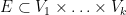
The factoring mentioned above is particularly simple in the case of proving Roth’s theorem, which is now presented separately in the above writeup.  Roth’s theorem seeks to locate a length three progression in which all three elements lie in a single set.  This will be deduced from an easier variant of the theorem in which one locates (a family of) length three progressions in which just the first two elements of the progression lie in a good set (and some other properties of the family are also required).  This is in turn derived from an even easier variant in which now just the first element of the progression is required to be in the good set.

More specifically, Roth’s theorem is now deduced from

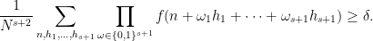
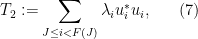
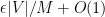
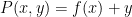
Theorem 1.5.  Let be a natural number, and let be a set of integers of upper density at least .  Then, whenever is partitioned into finitely many colour classes, there exists a colour class and a family of 3-term arithmetic progressions with the following properties:

1. For each , and lie in .
2. For each , lie in .
3. The for are in arithmetic progression.

The situation in this theorem is depicted by the following diagram, in which elements of are in blue and elements of are in grey:

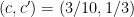
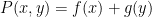
Theorem 1.5 is deduced in turn from the following easier variant:

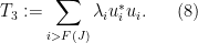
Theorem 1.6.  Let be a natural number, and let be a set of integers of upper density at least .  Then, whenever is partitioned into finitely many colour classes, there exists a colour class and a family of 3-term arithmetic progressions with the following properties:

1. For each , lie in .
2. For each , and lie in .
3. The for are in arithmetic progression.

The situation here is described by the figure below.

Theorem 1.6 is easy to prove.  To derive Theorem 1.5 from Theorem 1.6, or to derive Roth’s theorem from Theorem 1.5, one uses double counting arguments, van der Waerden’s theorem, and the weak regularity lemma, largely as described in this previous blog post; see the writeup for the full details.  (I would be interested in seeing a shorter proof of Theorem 1.5 though that did not go through these arguments, and did not use the more powerful theorems of  Roth or Szemerédi.)

 

An inverse theorem for the continuous Gowers uniformity norm

A few years ago, Ben Green, Tamar Ziegler, and myself proved the following (rather technical-looking) inverse theorem for the Gowers norms:

Theorem 1 (Discrete inverse theorem for Gowers norms) Let and be integers, and let . Suppose that is a function supported on such that

Then there exists a filtered nilmanifold of degree and complexity , a polynomial sequence , and a Lipschitz function of Lipschitz constant such that

For the definitions of “filtered nilmanifold”, “degree”, “complexity”, and “polynomial sequence”, see the paper of Ben, Tammy, and myself. (I should caution the reader that this blog post will presume a fair amount of familiarity with this subfield of additive combinatorics.) This result has a number of applications, for instance to establishing asymptotics for linear equations in the primes, but this will not be the focus of discussion here.

The purpose of this post is to record the observation that this “discrete” inverse theorem, together with an equidistribution theorem for nilsequences that Ben and I worked out in a separate paper, implies a continuous version:

Theorem 2 (Continuous inverse theorem for Gowers norms) Let be an integer, and let . Suppose that is a measurable function supported on such that

Then there exists a filtered nilmanifold of degree and complexity , a (smooth) polynomial sequence , and a Lipschitz function of Lipschitz constant such that

The interval can be easily replaced with any other fixed interval by a change of variables. A key point here is that the bounds are completely uniform in the choice of . Note though that the coefficients of can be arbitrarily large (and this is necessary, as can be seen just by considering functions of the form for some arbitrarily large frequency ).

It is likely that one could prove Theorem 2 by carefully going through the proof of Theorem 1 and replacing all instances of with (and making appropriate modifications to the argument to accommodate this). However, the proof of Theorem 1 is quite lengthy. Here, we shall proceed by the usual limiting process of viewing the continuous interval as a limit of the discrete interval as . However there will be some problems taking the limit due to a failure of compactness, and specifically with regards to the coefficients of the polynomial sequence produced by Theorem 1, after normalising these coefficients by . Fortunately, a factorisation theorem from a paper of Ben Green and myself resolves this problem by splitting into a “smooth” part which does enjoy good compactness properties, as well as “totally equidistributed” and “periodic” parts which can be eliminated using the measurability (and thus, approximate smoothness), of .

Ultraproducts as a Bridge Between Discrete and Continuous Analysis

(This is an extended blog post version of my talk “Ultraproducts as a Bridge Between Discrete and Continuous Analysis” that I gave at the Simons institute for the theory of computing at the workshop “Neo-Classical methods in discrete analysis“. Some of the material here is drawn from previous blog posts, notably “Ultraproducts as a bridge between hard analysis and soft analysis” and “Ultralimit analysis and quantitative algebraic geometry“‘. The text here has substantially more details than the talk; one may wish to skip all of the proofs given here to obtain a closer approximation to the original talk.)

Discrete analysis, of course, is primarily interested in the study of discrete (or “finitary”) mathematical objects: integers, rational numbers (which can be viewed as ratios of integers), finite sets, finite graphs, finite or discrete metric spaces, and so forth. However, many powerful tools in mathematics (e.g. ergodic theory, measure theory, topological group theory, algebraic geometry, spectral theory, etc.) work best when applied to continuous (or “infinitary”) mathematical objects: real or complex numbers, manifolds, algebraic varieties, continuous topological or metric spaces, etc. In order to apply results and ideas from continuous mathematics to discrete settings, there are basically two approaches. One is to directly discretise the arguments used in continuous mathematics, which often requires one to keep careful track of all the bounds on various quantities of interest, particularly with regard to various error terms arising from discretisation which would otherwise have been negligible in the continuous setting. The other is to construct continuous objects as limits of sequences of discrete objects of interest, so that results from continuous mathematics may be applied (often as a “black box”) to the continuous limit, which then can be used to deduce consequences for the original discrete objects which are quantitative (though often ineffectively so). The latter approach is the focus of this current talk.

The following table gives some examples of a discrete theory and its continuous counterpart, together with a limiting procedure that might be used to pass from the former to the latter:

(Discrete)	(Continuous)	(Limit method)
Ramsey theory	Topological dynamics	Compactness
Density Ramsey theory	Ergodic theory	Furstenberg correspondence principle
Graph/hypergraph regularity	Measure theory	Graph limits
Polynomial regularity	Linear algebra	Ultralimits
Structural decompositions	Hilbert space geometry	Ultralimits
Fourier analysis	Spectral theory	Direct and inverse limits
Quantitative algebraic geometry	Algebraic geometry	Schemes
Discrete metric spaces	Continuous metric spaces	Gromov-Hausdorff limits
Approximate group theory	Topological group theory	Model theory

As the above table illustrates, there are a variety of different ways to form a limiting continuous object. Roughly speaking, one can divide limits into three categories:

• Topological and metric limits. These notions of limits are commonly used by analysts. Here, one starts with a sequence (or perhaps a net) of objects in a common space , which one then endows with the structure of a topological space or a metric space, by defining a notion of distance between two points of the space, or a notion of open neighbourhoods or open sets in the space. Provided that the sequence or net is convergent, this produces a limit object , which remains in the same space, and is “close” to many of the original objects with respect to the given metric or topology.
• Categorical limits. These notions of limits are commonly used by algebraists. Here, one starts with a sequence (or more generally, a diagram) of objects in a category , which are connected to each other by various morphisms. If the ambient category is well-behaved, one can then form the direct limit or the inverse limit of these objects, which is another object in the same category , and is connected to the original objects by various morphisms.
• Logical limits. These notions of limits are commonly used by model theorists. Here, one starts with a sequence of objects or of spaces , each of which is (a component of) a model for given (first-order) mathematical language (e.g. if one is working in the language of groups, might be groups and might be elements of these groups). By using devices such as the ultraproduct construction, or the compactness theorem in logic, one can then create a new object or a new space , which is still a model of the same language (e.g. if the spaces were all groups, then the limiting space will also be a group), and is “close” to the original objects or spaces in the sense that any assertion (in the given language) that is true for the limiting object or space, will also be true for many of the original objects or spaces, and conversely. (For instance, if is an abelian group, then the will also be abelian groups for many .)

The purpose of this talk is to highlight the third type of limit, and specifically the ultraproduct construction, as being a “universal” limiting procedure that can be used to replace most of the limits previously mentioned. Unlike the topological or metric limits, one does not need the original objects to all lie in a common space in order to form an ultralimit ; they are permitted to lie in different spaces ; this is more natural in many discrete contexts, e.g. when considering graphs on vertices in the limit when goes to infinity. Also, no convergence properties on the are required in order for the ultralimit to exist. Similarly, ultraproduct limits differ from categorical limits in that no morphisms between the various spaces involved are required in order to construct the ultraproduct.

With so few requirements on the objects or spaces , the ultraproduct construction is necessarily a very “soft” one. Nevertheless, the construction has two very useful properties which make it particularly useful for the purpose of extracting good continuous limit objects out of a sequence of discrete objects. First of all, there is Łos’s theorem, which roughly speaking asserts that any first-order sentence which is asymptotically obeyed by the , will be exactly obeyed by the limit object ; in particular, one can often take a discrete sequence of “partial counterexamples” to some assertion, and produce a continuous “complete counterexample” that same assertion via an ultraproduct construction; taking the contrapositives, one can often then establish a rigorous equivalence between a quantitative discrete statement and its qualitative continuous counterpart. Secondly, there is the countable saturation property that ultraproducts automatically enjoy, which is a property closely analogous to that of compactness in topological spaces, and can often be used to ensure that the continuous objects produced by ultraproduct methods are “complete” or “compact” in various senses, which is particularly useful in being able to upgrade qualitative (or “pointwise”) bounds to quantitative (or “uniform”) bounds, more or less “for free”, thus reducing significantly the burden of “epsilon management” (although the price one pays for this is that one needs to pay attention to which mathematical objects of study are “standard” and which are “nonstandard”). To achieve this compactness or completeness, one sometimes has to restrict to the “bounded” portion of the ultraproduct, and it is often also convenient to quotient out the “infinitesimal” portion in order to complement these compactness properties with a matching “Hausdorff” property, thus creating familiar examples of continuous spaces, such as locally compact Hausdorff spaces.

Ultraproducts are not the only logical limit in the model theorist’s toolbox, but they are one of the simplest to set up and use, and already suffice for many of the applications of logical limits outside of model theory. In this post, I will set out the basic theory of these ultraproducts, and illustrate how they can be used to pass between discrete and continuous theories in each of the examples listed in the above table.

Apart from the initial “one-time cost” of setting up the ultraproduct machinery, the main loss one incurs when using ultraproduct methods is that it becomes very difficult to extract explicit quantitative bounds from results that are proven by transferring qualitative continuous results to the discrete setting via ultraproducts. However, in many cases (particularly those involving regularity-type lemmas) the bounds are already of tower-exponential type or worse, and there is arguably not much to be lost by abandoning the explicit quantitative bounds altogether.

The spectral proof of the Szemeredi regularity lemma

Perhaps the most important structural result about general large dense graphs is the Szemerédi regularity lemma. Here is a standard formulation of that lemma:

Lemma 1 (Szemerédi regularity lemma) Let be a graph on vertices, and let . Then there exists a partition for some with the property that for all but at most of the pairs , the pair is -regular in the sense that

whenever are such that and , and is the edge density between and . Furthermore, the partition is equitable in the sense that for all .

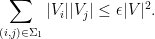
There are many proofs of this lemma, which is actually not that difficult to establish; see for instance these previous blog posts for some examples. In this post I would like to record one further proof, based on the spectral decomposition of the adjacency matrix of , which is essentially due to Frieze and Kannan. (Strictly speaking, Frieze and Kannan used a variant of this argument to establish a weaker form of the regularity lemma, but it is not difficult to modify the Frieze-Kannan argument to obtain the usual form of the regularity lemma instead. Some closely related spectral regularity lemmas were also developed by Szegedy.) I found recently (while speaking at the Abel conference in honour of this year’s laureate, Endre Szemerédi) that this particular argument is not as widely known among graph theory experts as I had thought, so I thought I would record it here.

For reasons of exposition, it is convenient to first establish a slightly weaker form of the lemma, in which one drops the hypothesis of equitability (but then has to weight the cells by their magnitude when counting bad pairs):

Lemma 2 (Szemerédi regularity lemma, weakened variant) . Let be a graph on vertices, and let . Then there exists a partition for some with the property that for all pairs outside of an exceptional set , one has

whenever , for some real number , where is the number of edges between and . Furthermore, we have

Let us now prove Lemma 2. We enumerate (after relabeling) as . The adjacency matrix of the graph is then a self-adjoint matrix, and thus admits an eigenvalue decomposition

for some orthonormal basis of and some eigenvalues , which we arrange in decreasing order of magnitude:

We can compute the trace of as

But we also have , so

Among other things, this implies that

for all .

Let be a function (depending on ) to be chosen later, with for all . Applying (3) and the pigeonhole principle (or the finite convergence principle, see this blog post), we can find such that

(Indeed, the bound on is basically iterated times.) We can now split

where is the “structured” component

is the “small” component

and is the “pseudorandom” component

We now design a vertex partition to make approximately constant on most cells. For each , we partition into cells on which (viewed as a function from to ) only fluctuates by , plus an exceptional cell of size coming from the values where is excessively large (larger than ). Combining all these partitions together, we can write for some , where has cardinality at most , and for all , the eigenfunctions all fluctuate by at most . In particular, if , then (by (4) and (6)) the entries of fluctuate by at most on each block . If we let be the mean value of these entries on , we thus have

for any and , where we view the indicator functions as column vectors of dimension .

Next, we observe from (3) and (7) that . If we let be the coefficients of , we thus have

and hence by Markov’s inequality we have

for all pairs 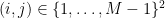outside of an exceptional set with

If avoids , we thus have

for any , by (10) and the Cauchy-Schwarz inequality.

Finally, to control we see from (4) and (8) that has an operator norm of at most . In particular, we have from the Cauchy-Schwarz inequality that

for any .

Let be the set of all pairs where either , , , or

One easily verifies that (2) holds. If is not in , then by summing (9), (11), (12) and using (5), we see that

for all . The left-hand side is just . As , we have

and so (since )

If we let be a sufficiently rapidly growing function of that depends on , the second error term in (13) can be absorbed in the first, and (1) follows. This concludes the proof of Lemma 2.

To prove Lemma 1, one argues similarly (after modifying as necessary), except that the initial partition of constructed above needs to be subdivided further into equitable components (of size ), plus some remainder sets which can be aggregated into an exceptional component of size (and which can then be redistributed amongst the other components to arrive at a truly equitable partition). We omit the details.

Remark 1 It is easy to verify that needs to be growing exponentially in in order for the above argument to work, which leads to tower-exponential bounds in the number of cells in the partition. It was shown by Gowers that a tower-exponential bound is actually necessary here. By varying , one basically obtains the strong regularity lemma first established by Alon, Fischer, Krivelevich, and Szegedy; in the opposite direction, setting essentially gives the weak regularity lemma of Frieze and Kannan.

Remark 2 If we specialise to a Cayley graph, in which is a finite abelian group and for some (symmetric) subset of , then the eigenvectors are characters, and one essentially recovers the arithmetic regularity lemma of Green, in which the vertex partition classes are given by Bohr sets (and one can then place additional regularity properties on these Bohr sets with some additional arguments). The components of , representing high, medium, and low eigenvalues of , then become a decomposition associated to high, medium, and low Fourier coefficients of .

Remark 3 The use of spectral theory here is parallel to the use of Fourier analysis to establish results such as Roth’s theorem on arithmetic progressions of length three. In analogy with this, one could view hypergraph regularity as being a sort of “higher order spectral theory”, although this spectral perspective is not as convenient as it is in the graph case.

Expanding polynomials over finite fields of large characteristic, and a regularity lemma for definable sets

I’ve just uploaded to the arXiv my paper “Expanding polynomials over finite fields of large characteristic, and a regularity lemma for definable sets“, submitted to Contrib. Disc. Math. The motivation of this paper is to understand a certain polynomial variant of the sum-product phenomenon in finite fields. This phenomenon asserts that if is a non-empty subset of a finite field , then either the sumset or product set will be significantly larger than , unless is close to a subfield of (or to ). In particular, in the regime when is large, say , one expects an expansion bound of the form

for some absolute constants . Results of this type are known; for instance, Hart, Iosevich, and Solymosi obtained precisely this bound for (in the case when is prime), which was then improved by Garaev to .

We have focused here on the case when is a large subset of , but sum-product estimates are also extremely interesting in the opposite regime in which is allowed to be small (see for instance the papers of Katz–Shen and Li and of Garaev for some recent work in this case, building on some older papers of Bourgain, Katz and myself and of Bourgain, Glibichuk, and Konyagin). However, the techniques used in these two regimes are rather different. For large subsets of , it is often profitable to use techniques such as the Fourier transform or the Cauchy-Schwarz inequality to “complete” a sum over a large set (such as ) into a set over the entire field , and then to use identities concerning complete sums (such as the Weil bound on complete exponential sums over a finite field). For small subsets of , such techniques are usually quite inefficient, and one has to proceed by somewhat different combinatorial methods which do not try to exploit the ambient field . But my paper focuses exclusively on the large regime, and unfortunately does not directly say much (except through reasoning by analogy) about the small case.

Note that it is necessary to have both and appear on the left-hand side of (1). Indeed, if one just has the sumset , then one can set to be a long arithmetic progression to give counterexamples to (1). Similarly, if one just has a product set , then one can set to be a long geometric progression. The sum-product phenomenon can then be viewed that it is not possible to simultaneously behave like a long arithmetic progression and a long geometric progression, unless one is already very close to behaving like a subfield.

Now we consider a polynomial variant of the sum-product phenomenon, where we consider a polynomial image

of a set with respect to a polynomial ; we can also consider the asymmetric setting of the image

of two subsets . The regime we will be interested is the one where the field is large, and the subsets of are also large, but the polynomial has bounded degree. Actually, for technical reasons it will not be enough for us to assume that has large cardinality; we will also need to assume that has large characteristic. (The two concepts are synonymous for fields of prime order, but not in general; for instance, the field with elements becomes large as while the characteristic remains fixed at , and is thus not going to be covered by the results in this paper.)

In this paper of Vu, it was shown that one could replace with in (1), thus obtaining a bound of the form

whenever for some absolute constants , unless the polynomial had the degenerate form for some linear function and polynomial , in which behaves too much like to get reasonable expansion. In this paper, we focus instead on the question of bounding alone. In particular, one can ask to classify the polynomials for which one has the weak expansion property

whenever for some absolute constants . One can also ask for stronger versions of this expander property, such as the moderate expansion property

whenever , or the almost strong expansion property

whenever . (One can consider even stronger expansion properties, such as the strong expansion property , but it was shown by Gyarmati and Sarkozy that this property cannot hold for polynomials of two variables of bounded degree when .) One can also consider asymmetric versions of these properties, in which one obtains lower bounds on rather than .

The example of a long arithmetic or geometric progression shows that the polynomials or cannot be expanders in any of the above senses, and a similar construction also shows that polynomials of the form or for some polynomials cannot be expanders. On the other hand, there are a number of results in the literature establishing expansion for various polynomials in two or more variables that are not of this degenerate form (in part because such results are related to incidence geometry questions in finite fields, such as the finite field version of the Erdos distinct distances problem). For instance, Solymosi established weak expansion for polynomials of the form when is a nonlinear polynomial, with generalisations by Hart, Li, and Shen for various polynomials of the form or . Further examples of expanding polynomials appear in the work of Shkredov, Iosevich-Rudnev, and Bukh-Tsimerman, as well as the previously mentioned paper of Vu and of Hart-Li-Shen, and these papers in turn cite many further results which are in the spirit of the polynomial expansion bounds discussed here (for instance, dealing with the small regime, or working in other fields such as instead of in finite fields ). We will not summarise all these results here; they are summarised briefly in my paper, and in more detail in the papers of Hart-Li-Shen and of Bukh-Tsimerman. But we will single out one of the results of Bukh-Tsimerman, which is one of most recent and general of these results, and closest to the results of my own paper. Roughly speaking, in this paper it is shown that a polynomial of two variables and bounded degree will be a moderate expander if it is non-composite (in the sense that it does not take the form for some non-linear polynomial and some polynomial , possibly having coefficients in the algebraic completion of ) and is monic on both and , thus it takes the form for some and some polynomial of degree at most in , and similarly with the roles of and reversed, unless is of the form or (in which case the expansion theory is covered to a large extent by the previous work of Hart, Li, and Shen).

Our first main result improves upon the Bukh-Tsimerman result by strengthening the notion of expansion and removing the non-composite and monic hypotheses, but imposes a condition of large characteristic. I’ll state the result here slightly informally as follows:

Theorem 1 (Criterion for moderate expansion) Let be a polynomial of bounded degree over a finite field of sufficiently large characteristic, and suppose that is not of the form or for some polynomials . Then one has the (asymmetric) moderate expansion property

whenever .

This is basically a sharp necessary and sufficient condition for asymmetric expansion moderate for polynomials of two variables. In the paper, analogous sufficient conditions for weak or almost strong expansion are also given, although these are not quite as satisfactory (particularly the conditions for almost strong expansion, which include a somewhat complicated algebraic condition which is not easy to check, and which I would like to simplify further, but was unable to).

The argument here resembles the Bukh-Tsimerman argument in many ways. One can view the result as an assertion about the expansion properties of the graph , which can essentially be thought of as a somewhat sparse three-uniform hypergraph on . Being sparse, it is difficult to directly apply techniques from dense graph or hypergraph theory for this situation; however, after a few applications of the Cauchy-Schwarz inequality, it turns out (as observed by Bukh and Tsimerman) that one can essentially convert the problem to one about the expansion properties of the set

(actually, one should view this as a multiset, but let us ignore this technicality) which one expects to be a dense set in , except in the case when the associated algebraic variety

fails to be Zariski dense, but it turns out that in this case one can use some differential geometry and Riemann surface arguments (after first invoking the Lefschetz principle and the high characteristic hypothesis to work over the complex numbers instead over a finite field) to show that is of the form or . This reduction is related to the classical fact that the only one-dimensional algebraic groups over the complex numbers are the additive group , the multiplicative group , or the elliptic curves (but the latter have a group law given by rational functions rather than polynomials, and so ultimately end up being eliminated from consideration, though they would play an important role if one wanted to study the expansion properties of rational functions).

It remains to understand the structure of the set (2) is. To understand dense graphs or hypergraphs, one of the standard tools of choice is the Szemerédi regularity lemma, which carves up such graphs into a bounded number of cells, with the graph behaving pseudorandomly on most pairs of cells. However, the bounds in this lemma are notoriously poor (the regularity obtained is an inverse tower exponential function of the number of cells), and this makes this lemma unsuitable for the type of expansion properties we seek (in which we want to deal with sets which have a polynomial sparsity, e.g. ). Fortunately, in the case of sets such as (2) which are definable over the language of rings, it turns out that a much stronger regularity lemma is available, which I call the “algebraic regularity lemma”. I’ll state it (again, slightly informally) in the context of graphs as follows:

Lemma 2 (Algebraic regularity lemma) Let be a finite field of large characteristic, and let be definable sets over of bounded complexity (i.e. are subsets of , for some bounded that can be described by some first-order predicate in the language of rings of bounded length and involving boundedly many constants). Let be a definable subset of , again of bounded complexity (one can view as a bipartite graph connecting and ). Then one can partition into a bounded number of cells , , still definable with bounded complexity, such that for all pairs , , one has the regularity property

for all , where is the density of in .

This lemma resembles the Szemerédi regularity lemma, but regularises all pairs of cells (not just most pairs), and the regularity is of polynomial strength in , rather than inverse tower exponential in the number of cells. Also, the cells are not arbitrary subsets of , but are themselves definable with bounded complexity, which turns out to be crucial for applications. I am optimistic that this lemma will be useful not just for studying expanding polynomials, but for many other combinatorial questions involving dense subsets of definable sets over finite fields.

The above lemma is stated for graphs , but one can iterate it to obtain an analogous regularisation of hypergraphs for any bounded (for application to (2), we need ). This hypergraph regularity lemma, by the way, is not analogous to the strong hypergraph regularity lemmas of Rodl et al. and Gowers developed in the last six or so years, but closer in spirit to the older (but weaker) hypergraph regularity lemma of Chung which gives the same “order ” regularity that the graph regularity lemma gives, rather than higher order regularity.

One feature of the proof of Lemma 2 which I found striking was the need to use some fairly high powered technology from algebraic geometry, and in particular the Lang-Weil bound on counting points in varieties over a finite field (discussed in this previous blog post), and also the theory of the etale fundamental group. Let me try to briefly explain why this is the case. A model example of a definable set of bounded complexity 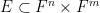is a set of the form

for some polynomial . (Actually, it turns out that one can essentially write all definable sets as an intersection of sets of this form; see this previous blog post for more discussion.) To regularise the set , it is convenient to square the adjacency matrix, which soon leads to the study of counting functions such as

If one can show that this function is “approximately finite rank” in the sense that (modulo lower order errors, of size smaller than the main term), this quantity depends only on a bounded number of bits of information about and a bounded number of bits of information about , then a little bit of linear algebra will then give the required regularity result.

One can recognise as counting -points of a certain algebraic variety

The Lang-Weil bound (discussed in this previous post) provides a formula for this count, in terms of the number of geometrically irreducible components of that are defined over (or equivalently, are invariant with respect to the Frobenius endomorphism associated to ). So the problem boils down to ensuring that this quantity is “generically bounded rank”, in the sense that for generic , its value depends only on a bounded number of bits of and a bounded number of bits of .

Here is where the étale fundamental group comes in. One can view as a fibre product of the varieties

and

over . If one is in sufficiently high characteristic (or even better, in zero characteristic, which one can reduce to by an ultraproduct (or nonstandard analysis) construction, similar to that discussed in this previous post), the varieties are generically finite étale covers of , and the fibre product is then also generically a finite étale cover. One can count the components of a finite étale cover of a connected variety by counting the number of orbits of the étale fundamental group acting on a fibre of that variety (much as the number of components of a cover of a connected manifold is the number of orbits of the topological fundamental group acting on that fibre). So if one understands the étale fundamental group of a certain generic subset of (formed by intersecting together an -dependent generic subset of with an -dependent generic subset), this in principle controls . It turns out that one can decouple the and dependence of this fundamental group by using an étale version of the van Kampen theorem for the fundamental group, which I discussed in this previous blog post. With this fact (and another deep fact about the étale fundamental group in zero characteristic, namely that it is topologically finitely generated), one can obtain the desired generic bounded rank property of , which gives the regularity lemma.

In order to expedite the deployment of all this algebraic geometry (as well as some Riemann surface theory), it is convenient to use the formalism of nonstandard analysis (or the ultraproduct construction), which among other things can convert quantitative, finitary problems in large characteristic into equivalent qualitative, infinitary problems in zero characteristic (in the spirit of this blog post). This allows one to use several tools from those fields as “black boxes”; not just the theory of étale fundamental groups (which are considerably simpler and more favorable in characteristic zero than they are in positive characteristic), but also some results limiting the morphisms between compact Riemann surfaces of high genus (such as the de Franchis theorem, the Riemann-Hurwitz formula, or the fact that all morphisms between elliptic curves are essentially group homomorphisms), which would be quite unwieldy to utilise if one did not first pass to the zero characteristic case (and thence to the complex case) via the ultraproduct construction (followed by the Lefschetz principle).

I found this project to be particularly educational for me, as it forced me to wander outside of my usual range by quite a bit in order to pick up the tools from algebraic geometry and Riemann surfaces that I needed (in particular, I read through several chapters of EGA and SGA for the first time). This did however put me in the slightly unnerving position of having to use results (such as the Riemann existence theorem) whose proofs I have not fully verified for myself, but which are easy to find in the literature, and widely accepted in the field. I suppose this type of dependence on results in the literature is more common in the more structured fields of mathematics than it is in analysis, which by its nature has fewer reusable black boxes, and so key tools often need to be rederived and modified for each new application. (This distinction is discussed further in this article of Gowers.)

An arithmetic regularity lemma, an associated counting lemma, and applications

Ben Green, and I have just uploaded to the arXiv our paper “An arithmetic regularity lemma, an associated counting lemma, and applications“, submitted (a little behind schedule) to the 70th birthday conference proceedings for Endre Szemerédi. In this paper we describe the general-degree version of the arithmetic regularity lemma, which can be viewed as the counterpart of the Szemerédi regularity lemma, in which the object being regularised is a function on a discrete interval rather than a graph, and the type of patterns one wishes to count are additive patterns (such as arithmetic progressions ) rather than subgraphs. Very roughly speaking, this regularity lemma asserts that all such functions can be decomposed as a degree nilsequence (or more precisely, a variant of a nilsequence that we call an virtual irrational nilsequence), plus a small error, plus a third error which is extremely tiny in the Gowers uniformity norm . In principle, at least, the latter two errors can be readily discarded in applications, so that the regularity lemma reduces many questions in additive combinatorics to questions concerning (virtual irrational) nilsequences. To work with these nilsequences, we also establish a arithmetic counting lemma that gives an integral formula for counting additive patterns weighted by such nilsequences.

The regularity lemma is a manifestation of the “dichotomy between structure and randomness”, as discussed for instance in my ICM article or FOCS article. In the degree case , this result is essentially due to Green. It is powered by the inverse conjecture for the Gowers norms, which we and Tamar Ziegler have recently established (paper to be forthcoming shortly; the case of our argument is discussed here). The counting lemma is established through the quantitative equidistribution theory of nilmanifolds, which Ben and I set out in this paper.

The regularity and counting lemmas are designed to be used together, and in the paper we give three applications of this combination. Firstly, we give a new proof of Szemerédi’s theorem, which proceeds via an energy increment argument rather than a density increment one. Secondly, we establish a conjecture of Bergelson, Host, and Kra, namely that if has density , and , then there exist shifts for which contains at least arithmetic progressions of length of spacing . (The case of this conjecture was established earlier by Green; the case is false, as was shown by Ruzsa in an appendix to the Bergelson-Host-Kra paper.) Thirdly, we establish a variant of a recent result of Gowers-Wolf, showing that the true complexity of a system of linear forms over indeed matches the conjectured value predicted in their first paper.

In all three applications, the scheme of proof can be described as follows:

• Apply the arithmetic regularity lemma, and decompose a relevant function into three pieces, .
• The uniform part is so tiny in the Gowers uniformity norm that its contribution can be easily dealt with by an appropriate “generalised von Neumann theorem”.
• The contribution of the (virtual, irrational) nilsequence can be controlled using the arithmetic counting lemma.
• Finally, one needs to check that the contribution of the small error does not overwhelm the main term . This is the trickiest bit; one often needs to use the counting lemma again to show that one can find a set of arithmetic patterns for that is so sufficiently “equidistributed” that it is not impacted by the small error.

To illustrate the last point, let us give the following example. Suppose we have a set of some positive density (say ) and we have managed to prove that contains a reasonable number of arithmetic progressions of length (say), e.g. it contains at least such progressions. Now we perturb by deleting a small number, say , elements from to create a new set . Can we still conclude that the new set contains any arithmetic progressions of length ?

Unfortunately, the answer could be no; conceivably, all of the arithmetic progressions in could be wiped out by the elements removed from , since each such element of could be associated with up to (or even ) arithmetic progressions in .

But suppose we knew that the arithmetic progressions in were equidistributed, in the sense that each element in belonged to the same number of such arithmetic progressions, namely . Then each element deleted from only removes at most progressions, and so one can safely remove elements from and still retain some arithmetic progressions. The same argument works if the arithmetic progressions are only approximately equidistributed, in the sense that the number of progressions that a given element belongs to concentrates sharply around its mean (for instance, by having a small variance), provided that the equidistribution is sufficiently strong. Fortunately, the arithmetic regularity and counting lemmas are designed to give precisely such a strong equidistribution result.

A succinct (but slightly inaccurate) summation of the regularity+counting lemma strategy would be that in order to solve a problem in additive combinatorics, it “suffices to check it for nilsequences”. But this should come with a caveat, due to the issue of the small error above; in addition to checking it for nilsequences, the answer in the nilsequence case must be sufficiently “dispersed” in a suitable sense, so that it can survive the addition of a small (but not completely negligible) perturbation.

One last “production note”. Like our previous paper with Emmanuel Breuillard, we used Subversion to write this paper, which turned out to be a significant efficiency boost as we could work on different parts of the paper simultaneously (this was particularly important this time round as the paper was somewhat lengthy and complicated, and there was a submission deadline). When doing so, we found it convenient to split the paper into a dozen or so pieces (one for each section of the paper, basically) in order to avoid conflicts, and to help coordinate the writing process. I’m also looking into git (a more advanced version control system), and am planning to use it for another of my joint projects; I hope to be able to comment on the relative strengths of these systems (and with plain old email) in the future.

Lewis lectures

This week I am at Rutgers University, giving the Lewis Memorial Lectures for this year, which are also concurrently part of a workshop in random matrices. I gave four lectures, three of which were on random matrices, and one of which was on the Szemerédi regularity lemma.

The titles, abstracts, and slides of these talks are as follows.

1. Szemerédi’s lemma revisited. In this general-audience talk, I discuss the Szemerédi regularity lemma (which, roughly speaking, shows that an arbitrary large dense graph can always be viewed as the disjoint union of a bounded number of pseudorandom components), and how it has recently been reinterpreted in a more analytical (and infinitary) language using the theory of graph limits or of exchangeable measures. I also discuss arithmetic analogues of this lemma, including one which (implicitly) underlies my result with Ben Green that the primes contain arbitrarily long arithmetic progressions.
2. Singularity and determinant of random matrices. Here, I present recent progress in understanding the question of how likely a random matrix (e.g. one whose entries are all +1 or -1 with equal probability) is to be invertible, as well as the related question of how large the determinant should be. The case of continuous matrix ensembles (such as the Gaussian ensemble) is well understood, but the discrete case contains some combinatorial difficulties and took longer to understand properly. In particular I present the results of Kahn-Komlós-Szemerédi and later authors showing that discrete random matrices are invertible with exponentially high probability, and also give some results for the distribution of the determinant.
3. The least singular value of random matrices. A more quantitative version of the question “when is a matrix invertible?” is “what is the least singular value of that matrix”? I present here the recent results of Litvak-Pajor-Rudelson-Tomczak-Jaegermann, Rudelson, myself and Vu, and Rudelson–Vershynin on addressing this question in the discrete case. A central role is played by the inverse Littlewood-Offord theorems of additive combinatorics, which give reasonably sharp necessary conditions for a discrete random walk to concentrate in a small ball.
4. The circular law. One interesting application of the above theory is to extend the circular law for the spectrum of random matrices from the continuous case to the discrete case. Previous arguments of Girko and Bai for the continuous case can be transplanted to the discrete case, but the key new ingredient needed is a least singular value bound for shifted matrices in order to avoid the spectrum being overwhelmed by pseudospectrum. It turns out that the results of the preceding lecture are almost precisely what are needed to accomplish this.

[Update, Mar 31: first lecture slides corrected.  Thanks to Yoshiyasu Ishigami for pointing out a slight inaccuracy in the text.]

On the testability and repair of hereditary hypergraph properties

I’ve just uploaded to the arXiv my joint paper with Tim Austin, “On the testability and repair of hereditary hypergraph properties“, which has been submitted to Random Structures and Algorithms. In this paper we prove some positive and negative results for the testability (and the local repairability) of various properties of directed or undirected graphs and hypergraphs, which can be either monochromatic or multicoloured.

The negative results have already been discussed in a previous posting of mine, so today I will focus on the positive results. The property testing results here are finitary results, but it turns out to be rather convenient to use a certain correspondence principle (the hypergraph version of the Furstenberg correspondence principle) to convert the question into one about exchangeable probability measures on spaces of hypergraphs (i.e. on random hypergraphs whose probability distribution is invariant under exchange of vertices). Such objects are also closely related to the”graphons” and “hypergraphons” that emerge as graph limits, as studied by Lovasz-Szegedy, Elek-Szegedy, and others. Somewhat amusingly, once one does so, it then becomes convenient to keep track of objects indexed by vertex sets and how they are exchanged via the language of category theory, and in particular using the concept of a natural transformation to describe such objects as exchangeable measures, graph colourings, and local modification rules. I will try to sketch out some of these connections, after describing the main positive results.

The Lebesgue differentiation theorem and the Szemeredi regularity lemma

This post is a sequel of sorts to my earlier post on hard and soft analysis, and the finite convergence principle. Here, I want to discuss a well-known theorem in infinitary soft analysis – the Lebesgue differentiation theorem – and whether there is any meaningful finitary version of this result. Along the way, it turns out that we will uncover a simple analogue of the Szemerédi regularity lemma, for subsets of the interval rather than for graphs. (Actually, regularity lemmas seem to appear in just about any context in which fine-scaled objects can be approximated by coarse-scaled ones.) The connection between regularity lemmas and results such as the Lebesgue differentiation theorem was recently highlighted by Elek and Szegedy, while the connection between the finite convergence principle and results such as the pointwise ergodic theorem (which is a close cousin of the Lebesgue differentiation theorem) was recently detailed by Avigad, Gerhardy, and Towsner.

The Lebesgue differentiation theorem has many formulations, but we will avoid the strongest versions and just stick to the following model case for simplicity:

Lebesgue differentiation theorem. If is Lebesgue measurable, then for almost every we have . Equivalently, the fundamental theorem of calculus is true for almost every x in [0,1].

Here we use the oriented definite integral, thus . Specialising to the case where is an indicator function, we obtain the Lebesgue density theorem as a corollary:

Lebesgue density theorem. Let be Lebesgue measurable. Then for almost every , we have as , where |A| denotes the Lebesgue measure of A.

In other words, almost all the points x of A are points of density of A, which roughly speaking means that as one passes to finer and finer scales, the immediate vicinity of x becomes increasingly saturated with A. (Points of density are like robust versions of interior points, thus the Lebesgue density theorem is an assertion that measurable sets are almost like open sets. This is Littlewood’s first principle.) One can also deduce the Lebesgue differentiation theorem back from the Lebesgue density theorem by approximating f by a finite linear combination of indicator functions; we leave this as an exercise.

Simons Lecture II: Structure and randomness in ergodic theory and graph theory

In this second lecture, I wish to talk about the dichotomy between structure and randomness as it manifests itself in four closely related areas of mathematics:

• Combinatorial number theory, which seeks to find patterns in unstructured dense sets (or colourings) of integers;
• Ergodic theory (or more specifically, multiple recurrence theory), which seeks to find patterns in positive-measure sets under the action of a discrete dynamical system on probability spaces (or more specifically, measure-preserving actions of the integers );
• Graph theory, or more specifically the portion of this theory concerned with finding patterns in large unstructured dense graphs; and
• Ergodic graph theory, which is a very new and undeveloped subject, which roughly speaking seems to be concerned with the patterns within a measure-preserving action of the infinite permutation group , which is one of several models we have available to study infinite “limits” of graphs.

The two “discrete” (or “finitary”, or “quantitative”) fields of combinatorial number theory and graph theory happen to be related to each other, basically by using the Cayley graph construction; I will give an example of this shortly. The two “continuous” (or “infinitary”, or “qualitative”) fields of ergodic theory and ergodic graph theory are at present only related on the level of analogy and informal intuition, but hopefully some more systematic connections between them will appear soon.

On the other hand, we have some very rigorous connections between combinatorial number theory and ergodic theory, and also (more recently) between graph theory and ergodic graph theory, basically by the procedure of viewing the infinitary continuous setting as a limit of the finitary discrete setting. These two connections go by the names of the Furstenberg correspondence principle and the graph correspondence principle respectively. These principles allow one to tap the power of the infinitary world (for instance, the ability to take limits and perform completions or closures of objects) in order to establish results in the finitary world, or at least to take the intuition gained in the infinitary world and transfer it to a finitary setting. Conversely, the finitary world provides an excellent model setting to refine one’s understanding of infinitary objects, for instance by establishing quantitative analogues of “soft” results obtained in an infinitary manner. I will remark here that this best-of-both-worlds approach, borrowing from both the finitary and infinitary traditions of mathematics, was absolutely necessary for Ben Green and I in order to establish our result on long arithmetic progressions in the primes. In particular, the infinitary setting is excellent for being able to rigorously define and study concepts (such as structure or randomness) which are much “fuzzier” and harder to pin down exactly in the finitary world.