You are currently browsing the category archive for the ‘math.IT’ category.

A family {A_1,\dots,A_r} of sets for some {r \geq 1} is a sunflower if there is a core set {A_0} contained in each of the {A_i} such that the petal sets {A_i \backslash A_0, i=1,\dots,r} are disjoint. If {k,r \geq 1}, let {\mathrm{Sun}(k,r)} denote the smallest natural number with the property that any family of {\mathrm{Sun}(k,r)} distinct sets of cardinality at most {k} contains {r} distinct elements {A_1,\dots,A_r} that form a sunflower. The celebrated Erdös-Rado theorem asserts that {\mathrm{Sun}(k,r)} is finite; in fact Erdös and Rado gave the bounds

\displaystyle  (r-1)^k \leq \mathrm{Sun}(k,r) \leq (r-1)^k k! + 1. \ \ \ \ \ (1)

The sunflower conjecture asserts in fact that the upper bound can be improved to {\mathrm{Sun}(k,r) \leq O(1)^k r^k}. This remains open at present despite much effort (including a Polymath project); after a long series of improvements to the upper bound, the best general bound known currently is

\displaystyle  \mathrm{Sun}(k,r) \leq O( r \log(kr) )^k \ \ \ \ \ (2)

for all {k,r \geq 2}, established in 2019 by Rao (building upon a recent breakthrough a month previously of Alweiss, Lovett, Wu, and Zhang). Here we remove the easy cases {k=1} or {r=1} in order to make the logarithmic factor {\log(kr)} a little cleaner.

Rao’s argument used the Shannon noiseless coding theorem. It turns out that the argument can be arranged in the very slightly different language of Shannon entropy, and I would like to present it here. The argument proceeds by locating the core and petals of the sunflower separately (this strategy is also followed in Alweiss-Lovett-Wu-Zhang). In both cases the following definition will be key. In this post all random variables, such as random sets, will be understood to be discrete random variables taking values in a finite range. We always use boldface symbols to denote random variables, and non-boldface for deterministic quantities.

Definition 1 (Spread set) Let {R > 1}. A random set {{\bf A}} is said to be {R}-spread if one has

\displaystyle  {\mathbb P}( S \subset {\bf A}) \leq R^{-|S|}

for all sets {S}. A family {(A_i)_{i \in I}} of sets is said to be {R}-spread if {I} is non-empty and the random variable {A_{\bf i}} is {R}-spread, where {{\bf i}} is drawn uniformly from {I}.

The core can then be selected greedily in such a way that the remainder of a family becomes spread:

Lemma 2 (Locating the core) Let {(A_i)_{i \in I}} be a family of subsets of a finite set {X}, each of cardinality at most {k}, and let {R > 1}. Then there exists a “core” set {S_0} of cardinality at most {k} such that the set

\displaystyle  J := \{ i \in I: S_0 \subset A_i \} \ \ \ \ \ (3)

has cardinality at least {R^{-|S_0|} |I|}, and such that the family {(A_j \backslash S_0)_{j \in J}} is {R}-spread. Furthermore, if {|I| > R^k} and the {A_i} are distinct, then {|S_0| < k}.

Proof: We may assume {I} is non-empty, as the claim is trivial otherwise. For any {S \subset X}, define the quantity

\displaystyle  Q(S) := R^{|S|} |\{ i \in I: S \subset A_i\}|,

and let {S_0} be a subset of {X} that maximizes {Q(S_0)}. Since {Q(\emptyset) = |I| > 0} and {Q(S)=0} when {|S| >k}, we see that {0 \leq |S_0| \leq K}. If the {A_i} are distinct and {|I| > R^k}, then we also have {Q(S) \leq R^k < |I| = Q(\emptyset)} when {|S|=k}, thus in this case we have {|S_0| < k}.

Let {J} be the set (3). Since {Q(S_0) \geq Q(\emptyset)>0}, {J} is non-empty. It remains to check that the family {(A_j \backslash S_0)_{j \in J}} is {R}-spread. But for any {S \subset X} and {{\bf j}} drawn uniformly at random from {J} one has

\displaystyle  {\mathbb P}( S \subset A_{\bf j} \backslash S_0 ) = \frac{|\{ i \in I: S_0 \cup S \subset A_i\}|}{|\{ i \in I: S_0 \subset A_i\}|} = R^{|S_0|-|S_0 \cup S|} \frac{Q(S)}{Q(S_0)}.

Observe that {Q(S) \leq Q(S_0)}, and the probability is only non-empty when {S, S_0} are disjoint, so that {|S_0|-|S_0 \cup S| = - |S|}. The claim follows. \Box

In view of the above lemma, the bound (2) will then follow from

Proposition 3 (Locating the petals) Let {r, k \geq 2} be natural numbers, and suppose that {R \geq C r \log(kr)} for a sufficiently large constant {C}. Let {(A_i)_{i \in I}} be a finite family of subsets of a finite set {X}, each of cardinality at most {k} which is {R}-spread. Then there exist {i_1,\dots,i_r \in I} such that {A_{i_1},\dots,A_{i_r}} is disjoint.

Indeed, to prove (2), we assume that {(A_i)_{i \in I}} is a family of sets of cardinality greater than {R^k} for some {R \geq Cr \log(kr)}; by discarding redundant elements and sets we may assume that {I} is finite and that all the {A_i} are contained in a common finite set {X}. Apply Lemma 2 to find a set {S_0 \subset X} of cardinality {|S_0| < k} such that the family {(A_j \backslash S_0)_{j \in J}} is {R}-spread. By Proposition 3 we can find {j_1,\dots,j_r \in J} such that {A_{j_1} \backslash S_0,\dots,A_{j_r} \backslash S_0} are disjoint; since these sets have cardinality {k - |S_0| > 0}, this implies that the {j_1,\dots,j_r} are distinct. Hence {A_{j_1},\dots,A_{j_r}} form a sunflower as required.

Remark 4 Proposition 3 is easy to prove if we strengthen the condition on {R} to {R > k(r-1)}. In this case, we have {\mathop{\bf P}_{i \in I}( x \in A_i) < 1/k(r-1)} for every {x \in X}, hence by the union bound we see that for any {i_1,\dots,i_j \in I} with {j \leq r-1} there exists {i_{j+1} \in I} such that {A_{i_{j+1}}} is disjoint from the set {A_{i_1} \cup \dots \cup A_{i_j}}, which has cardinality at most {k(r-1)}. Iterating this, we obtain the conclusion of Proposition 3 in this case. This recovers a bound of the form {\mathrm{Sun}(k,r) \leq (k(r-1))^k+1}, and by pursuing this idea a little further one can recover the original upper bound (1) of Erdös and Rado.

It remains to prove Proposition 3. In fact we can locate the petals one at a time, placing each petal inside a random set.

Proposition 5 (Locating a single petal) Let the notation and hypotheses be as in Proposition 3. Let {{\bf V}} be a random subset of {X}, such that each {x \in X} lies in {{\bf V}} with an independent probability of {1/r}. Then with probability greater than {1-1/r}, {{\bf V}} contains one of the {A_i}.

To see that Proposition 5 implies Proposition 3, we randomly partition {X} into {{\bf V}_1 \cup \dots \cup {\bf V}_r} by placing each {x \in X} into one of the {{\bf V}_j}, {j=1,\dots,r} chosen uniformly and independently at random. By Proposition 5 and the union bound, we see that with positive probability, it is simultaneously true for all {j=1,\dots,r} that each {{\bf V}_j} contains one of the {A_i}. Selecting one such {A_i} for each {{\bf V}_j}, we obtain the required disjoint petals.

We will prove Proposition 5 by gradually increasing the density of the random set and arranging the sets {A_i} to get quickly absorbed by this random set. The key iteration step is

Proposition 6 (Refinement inequality) Let {R > 1} and {0 < \delta < 1}. Let {{\bf A}} be a random subset of a finite set {X} which is {R}-spread, and let {{\bf V}} be a random subset of {X} independent of {{\bf A}}, such that each {x \in X} lies in {{\bf V}} with an independent probability of {\delta}. Then there exists another {R}-spread random subset {{\bf A}'} of {X} whose support is contained in the support of {{\bf A}}, such that {{\bf A}' \backslash {\bf V} \subset {\bf A}} and

\displaystyle  {\mathbb E} |{\bf A}' \backslash {\bf V}| \leq \frac{5}{\log(R\delta)} {\mathbb E} |{\bf A}|.

Note that a direct application of the first moment method gives only the bound

\displaystyle  {\mathbb E} |{\bf A} \backslash {\bf V}| \leq (1-\delta) {\mathbb E} |{\bf A}|,

but the point is that by switching from {{\bf A}} to an equivalent {{\bf A}'} we can replace the {1-\delta} factor by a quantity significantly smaller than {1}.

One can iterate the above proposition, repeatedly replacing {{\bf A}, X} with {{\bf A}' \backslash {\bf V}, X \backslash {\bf V}} (noting that this preserves the {R}-spread nature of {{\bf A}}) to conclude

Corollary 7 (Iterated refinement inequality) Let {R > 1}, {0 < \delta < 1}, and {m \geq 1}. Let {{\bf A}} be a random subset of a finite set {X} which is {R}-spread, and let {{\bf V}} be a random subset of {X} independent of {{\bf A}}, such that each {x \in X} lies in {{\bf V}} with an independent probability of {1-(1-\delta)^m}. Then there exists another random subset {{\bf A}'} of {X} with support contained in the support of {{\bf A}}, such that

\displaystyle  {\mathbb E} |{\bf A}' \backslash {\bf V}| \leq (\frac{5}{\log(R\delta)})^m {\mathbb E} |{\bf A}|.

Now we can prove Proposition 5. Let {m} be chosen shortly. Applying Corollary 7 with {{\bf A}} drawn uniformly at random from the {(A_i)_{i \in I}}, and setting {1-(1-\delta)^m = 1/r}, or equivalently {\delta = 1 - (1 - 1/r)^{1/m}}, we have

\displaystyle  {\mathbb E} |{\bf A}' \backslash {\bf V}| \leq (\frac{5}{\log(R\delta)})^m k.

In particular, if we set {m = \lceil \log kr \rceil}, so that {\delta \sim \frac{1}{r \log kr}}, then by choice of {R} we have {\frac{5}{\log(R\delta)} < \frac{1}{2}}, hence

\displaystyle  {\mathbb E} |{\bf A}' \backslash {\bf V}| < \frac{1}{r}.

In particular with probability at least {1 - \frac{1}{r}}, there must exist {A_i} such that {|A_i \backslash {\bf V}| = 0}, giving the proposition.

It remains to establish Proposition 6. This is the difficult step, and requires a clever way to find the variant {{\bf A}'} of {{\bf A}} that has better containment properties in {{\bf V}} than {{\bf A}} does. The main trick is to make a conditional copy {({\bf A}', {\bf V}')} of {({\bf A}, {\bf V})} that is conditionally independent of {({\bf A}, {\bf V})} subject to the constraint {{\bf A} \cup {\bf V} = {\bf A}' \cup {\bf V}'}. The point here is that this constrant implies the inclusions

\displaystyle  {\bf A}' \backslash {\bf V} \subset {\bf A} \cap {\bf A}' \subset {\bf A} \ \ \ \ \ (4)

and

\displaystyle  {\bf A}' \backslash {\bf A} \subset {\bf V}. \ \ \ \ \ (5)

Because of the {R}-spread hypothesis, it is hard for {{\bf A}} to contain any fixed large set. If we could apply this observation in the contrapositive to {{\bf A} \cap {\bf A}'} we could hope to get a good upper bound on the size of {{\bf A} \cap {\bf A}'} and hence on {{\bf A} \backslash {\bf V}} thanks to (4). One can also hope to improve such an upper bound by also employing (5), since it is also hard for the random set {{\bf V}} to contain a fixed large set. There are however difficulties with implementing this approach due to the fact that the random sets {{\bf A} \cap {\bf A}', {\bf A}' \backslash {\bf A}} are coupled with {{\bf A}, {\bf V}} in a moderately complicated fashion. In Rao’s argument a somewhat complicated encoding scheme was created to give information-theoretic control on these random variables; below the fold we accomplish a similar effect by using Shannon entropy inequalities in place of explicit encoding. A certain amount of information-theoretic sleight of hand is required to decouple certain random variables to the extent that the Shannon inequalities can be effectively applied. The argument bears some resemblance to the “entropy compression method” discussed in this previous blog post; there may be a way to more explicitly express the argument below in terms of that method. (There is also some kinship with the method of dependent random choice, which is used for instance to establish the Balog-Szemerédi-Gowers lemma, and was also translated into information theoretic language in these unpublished notes of Van Vu and myself.)

Read the rest of this entry »

In these notes we presume familiarity with the basic concepts of probability theory, such as random variables (which could take values in the reals, vectors, or other measurable spaces), probability, and expectation. Much of this theory is in turn based on measure theory, which we will also presume familiarity with. See for instance this previous set of lecture notes for a brief review.

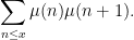
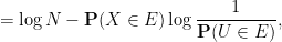
The basic objects of study in analytic number theory are deterministic; there is nothing inherently random about the set of prime numbers, for instance. Despite this, one can still interpret many of the averages encountered in analytic number theory in probabilistic terms, by introducing random variables into the subject. Consider for instance the form

\displaystyle \sum_{n \leq x} \mu(n) = o(x) \ \ \ \ \ (1)


of the prime number theorem (where we take the limit {x \rightarrow \infty}). One can interpret this estimate probabilistically as

\displaystyle {\mathbb E} \mu(\mathbf{n}) = o(1) \ \ \ \ \ (2)

where {\mathbf{n} = \mathbf{n}_{\leq x}} is a random variable drawn uniformly from the natural numbers up to {x}, and {{\mathbb E}} denotes the expectation. (In this set of notes we will use boldface symbols to denote random variables, and non-boldface symbols for deterministic objects.) By itself, such an interpretation is little more than a change of notation. However, the power of this interpretation becomes more apparent when one then imports concepts from probability theory (together with all their attendant intuitions and tools), such as independence, conditioning, stationarity, total variation distance, and entropy. For instance, suppose we want to use the prime number theorem (1) to make a prediction for the sum

\displaystyle \sum_{n \leq x} \mu(n) \mu(n+1).

After dividing by {x}, this is essentially

\displaystyle {\mathbb E} \mu(\mathbf{n}) \mu(\mathbf{n}+1).

With probabilistic intuition, one may expect the random variables {\mu(\mathbf{n}), \mu(\mathbf{n}+1)} to be approximately independent (there is no obvious relationship between the number of prime factors of {\mathbf{n}}, and of {\mathbf{n}+1}), and so the above average would be expected to be approximately equal to

\displaystyle ({\mathbb E} \mu(\mathbf{n})) ({\mathbb E} \mu(\mathbf{n}+1))

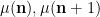
which by (2) is equal to {o(1)}. Thus we are led to the prediction

\displaystyle \sum_{n \leq x} \mu(n) \mu(n+1) = o(x). \ \ \ \ \ (3)

The asymptotic (3) is widely believed (it is a special case of the Chowla conjecture, which we will discuss in later notes; while there has been recent progress towards establishing it rigorously, it remains open for now.
How would one try to make these probabilistic intuitions more rigorous? The first thing one needs to do is find a more quantitative measurement of what it means for two random variables to be “approximately” independent. There are several candidates for such measurements, but we will focus in these notes on two particularly convenient measures of approximate independence: the “{L^2}” measure of independence known as covariance, and the “{L \log L}” measure of independence known as mutual information (actually we will usually need the more general notion of conditional mutual information that measures conditional independence). The use of {L^2} type methods in analytic number theory is well established, though it is usually not described in probabilistic terms, being referred to instead by such names as the “second moment method”, the “large sieve” or the “method of bilinear sums”. The use of {L \log L} methods (or “entropy methods”) is much more recent, and has been able to control certain types of averages in analytic number theory that were out of reach of previous methods such as {L^2} methods. For instance, in later notes we will use entropy methods to establish the logarithmically averaged version

\displaystyle \sum_{n \leq x} \frac{\mu(n) \mu(n+1)}{n} = o(\log x) \ \ \ \ \ (4)


of (3), which is implied by (3) but strictly weaker (much as the prime number theorem (1) implies the bound {\sum_{n \leq x} \frac{\mu(n)}{n} = o(\log x)}, but the latter bound is much easier to establish than the former).
As with many other situations in analytic number theory, we can exploit the fact that certain assertions (such as approximate independence) can become significantly easier to prove if one only seeks to establish them on average, rather than uniformly. For instance, given two random variables {\mathbf{X}} and {\mathbf{Y}} of number-theoretic origin (such as the random variables {\mu(\mathbf{n})} and {\mu(\mathbf{n}+1)} mentioned previously), it can often be extremely difficult to determine the extent to which {\mathbf{X},\mathbf{Y}} behave “independently” (or “conditionally independently”). However, thanks to second moment tools or entropy based tools, it is often possible to assert results of the following flavour: if {\mathbf{Y}_1,\dots,\mathbf{Y}_k} are a large collection of “independent” random variables, and {\mathbf{X}} is a further random variable that is “not too large” in some sense, then {\mathbf{X}} must necessarily be nearly independent (or conditionally independent) to many of the {\mathbf{Y}_i}, even if one cannot pinpoint precisely which of the {\mathbf{Y}_i} the variable {\mathbf{X}} is independent with. In the case of the second moment method, this allows us to compute correlations such as {{\mathbb E} {\mathbf X} \mathbf{Y}_i} for “most” {i}. The entropy method gives bounds that are significantly weaker quantitatively than the second moment method (and in particular, in its current incarnation at least it is only able to say non-trivial assertions involving interactions with residue classes at small primes), but can control significantly more general quantities {{\mathbb E} F( {\mathbf X}, \mathbf{Y}_i )} for “most” {i} thanks to tools such as the Pinsker inequality.

Read the rest of this entry »

Just a short post to note that Norwegian Academy of Science and Letters has just announced that the 2017 Abel prize has been awarded to Yves Meyer, “for his pivotal role in the development of the mathematical theory of wavelets”.  The actual prize ceremony will be at Oslo in May.

I am actually in Oslo myself currently, having just presented Meyer’s work at the announcement ceremony (and also having written a brief description of some of his work).  The Abel prize has a somewhat unintuitive (and occasionally misunderstood) arrangement in which the presenter of the work of the prize is selected independently of the winner of the prize (I think in part so that the choice of presenter gives no clues as to the identity of the laureate).  In particular, like other presenters before me (which in recent years have included Timothy Gowers, Jordan Ellenberg, and Alex Bellos), I agreed to present the laureate’s work before knowing who the laureate was!  But in this case the task was very easy, because Meyer’s areas of (both pure and applied) harmonic analysis and PDE fell rather squarely within my own area of expertise.  (I had previously written about some other work of Meyer in this blog post.)  Indeed I had learned about Meyer’s wavelet constructions as a graduate student while taking a course from Ingrid Daubechies.   Daubechies also made extremely important contributions to the theory of wavelets, but due to a conflict of interest (as per the guidelines for the prize committee) arising from Daubechies’ presidency of the International Mathematical Union (which nominates the majority of the members of the Abel prize committee, who then serve for two years) from 2011 to 2014 (and her continuing service ex officio on the IMU executive committee from 2015 to 2018), she will not be eligible for the prize until 2021 at the earliest, and so I do not think this prize should be necessarily construed as a judgement on the relative contributions of Meyer and Daubechies to this field.  (In any case I fully agree with the Abel prize committee’s citation of Meyer’s pivotal role in the development of the theory of wavelets.)

[Update, Mar 28: link to prize committee guidelines and clarification of the extent of Daubechies’ conflict of interest added. -T]

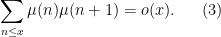
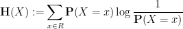
Given a random variable {X} that takes on only finitely many values, we can define its Shannon entropy by the formula

\displaystyle H(X) := \sum_x \mathbf{P}(X=x) \log \frac{1}{\mathbf{P}(X=x)}

with the convention that {0 \log \frac{1}{0} = 0}. (In some texts, one uses the logarithm to base {2} rather than the natural logarithm, but the choice of base will not be relevant for this discussion.) This is clearly a nonnegative quantity. Given two random variables {X,Y} taking on finitely many values, the joint variable {(X,Y)} is also a random variable taking on finitely many values, and also has an entropy {H(X,Y)}. It obeys the Shannon inequalities

\displaystyle H(X), H(Y) \leq H(X,Y) \leq H(X) + H(Y)

so we can define some further nonnegative quantities, the mutual information

\displaystyle I(X:Y) := H(X) + H(Y) - H(X,Y)

and the conditional entropies

\displaystyle H(X|Y) := H(X,Y) - H(Y); \quad H(Y|X) := H(X,Y) - H(X).

More generally, given three random variables {X,Y,Z}, one can define the conditional mutual information

\displaystyle I(X:Y|Z) := H(X|Z) + H(Y|Z) - H(X,Y|Z)

and the final of the Shannon entropy inequalities asserts that this quantity is also non-negative.

The mutual information {I(X:Y)} is a measure of the extent to which {X} and {Y} fail to be independent; indeed, it is not difficult to show that {I(X:Y)} vanishes if and only if {X} and {Y} are independent. Similarly, {I(X:Y|Z)} vanishes if and only if {X} and {Y} are conditionally independent relative to {Z}. At the other extreme, {H(X|Y)} is a measure of the extent to which {X} fails to depend on {Y}; indeed, it is not difficult to show that {H(X|Y)=0} if and only if {X} is determined by {Y} in the sense that there is a deterministic function {f} such that {X = f(Y)}. In a related vein, if {X} and {X'} are equivalent in the sense that there are deterministic functional relationships {X = f(X')}, {X' = g(X)} between the two variables, then {X} is interchangeable with {X'} for the purposes of computing the above quantities, thus for instance {H(X) = H(X')}, {H(X,Y) = H(X',Y)}, {I(X:Y) = I(X':Y)}, {I(X:Y|Z) = I(X':Y|Z)}, etc..

One can get some initial intuition for these information-theoretic quantities by specialising to a simple situation in which all the random variables {X} being considered come from restricting a single random (and uniformly distributed) boolean function {F: \Omega \rightarrow \{0,1\}} on a given finite domain {\Omega} to some subset {A} of {\Omega}:

\displaystyle X = F \downharpoonright_A.

In this case, {X} has the law of a random uniformly distributed boolean function from {A} to {\{0,1\}}, and the entropy here can be easily computed to be {|A| \log 2}, where {|A|} denotes the cardinality of {A}. If {X} is the restriction of {F} to {A}, and {Y} is the restriction of {F} to {B}, then the joint variable {(X,Y)} is equivalent to the restriction of {F} to {A \cup B}. If one discards the normalisation factor {\log 2}, one then obtains the following dictionary between entropy and the combinatorics of finite sets:

Random variables {X,Y,Z} Finite sets {A,B,C}
Entropy {H(X)} Cardinality {|A|}
Joint variable {(X,Y)} Union {A \cup B}
Mutual information {I(X:Y)} Intersection cardinality {|A \cap B|}
Conditional entropy {H(X|Y)} Set difference cardinality {|A \backslash B|}
Conditional mutual information {I(X:Y|Z)} {|(A \cap B) \backslash C|}
{X, Y} independent {A, B} disjoint
{X} determined by {Y} {A} a subset of {B}
{X,Y} conditionally independent relative to {Z} {A \cap B \subset C}

Every (linear) inequality or identity about entropy (and related quantities, such as mutual information) then specialises to a combinatorial inequality or identity about finite sets that is easily verified. For instance, the Shannon inequality {H(X,Y) \leq H(X)+H(Y)} becomes the union bound {|A \cup B| \leq |A| + |B|}, and the definition of mutual information becomes the inclusion-exclusion formula

\displaystyle |A \cap B| = |A| + |B| - |A \cup B|.

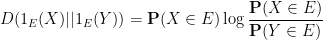
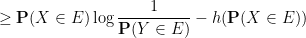
For a more advanced example, consider the data processing inequality that asserts that if {X, Z} are conditionally independent relative to {Y}, then {I(X:Z) \leq I(X:Y)}. Specialising to sets, this now says that if {A, C} are disjoint outside of {B}, then {|A \cap C| \leq |A \cap B|}; this can be made apparent by considering the corresponding Venn diagram. This dictionary also suggests how to prove the data processing inequality using the existing Shannon inequalities. Firstly, if {A} and {C} are not necessarily disjoint outside of {B}, then a consideration of Venn diagrams gives the more general inequality

\displaystyle |A \cap C| \leq |A \cap B| + |(A \cap C) \backslash B|

and a further inspection of the diagram then reveals the more precise identity

\displaystyle |A \cap C| + |(A \cap B) \backslash C| = |A \cap B| + |(A \cap C) \backslash B|.

Using the dictionary in the reverse direction, one is then led to conjecture the identity

\displaystyle I( X : Z ) + I( X : Y | Z ) = I( X : Y ) + I( X : Z | Y )

which (together with non-negativity of conditional mutual information) implies the data processing inequality, and this identity is in turn easily established from the definition of mutual information.

On the other hand, not every assertion about cardinalities of sets generalises to entropies of random variables that are not arising from restricting random boolean functions to sets. For instance, a basic property of sets is that disjointness from a given set {C} is preserved by unions:

\displaystyle A \cap C = B \cap C = \emptyset \implies (A \cup B) \cap C = \emptyset.

Indeed, one has the union bound

\displaystyle |(A \cup B) \cap C| \leq |A \cap C| + |B \cap C|. \ \ \ \ \ (1)

Applying the dictionary in the reverse direction, one might now conjecture that if {X} was independent of {Z} and {Y} was independent of {Z}, then {(X,Y)} should also be independent of {Z}, and furthermore that

\displaystyle I(X,Y:Z) \leq I(X:Z) + I(Y:Z)

but these statements are well known to be false (for reasons related to pairwise independence of random variables being strictly weaker than joint independence). For a concrete counterexample, one can take {X, Y \in {\bf F}_2} to be independent, uniformly distributed random elements of the finite field {{\bf F}_2} of two elements, and take {Z := X+Y} to be the sum of these two field elements. One can easily check that each of {X} and {Y} is separately independent of {Z}, but the joint variable {(X,Y)} determines {Z} and thus is not independent of {Z}.

From the inclusion-exclusion identities

\displaystyle |A \cap C| = |A| + |C| - |A \cup C|

\displaystyle |B \cap C| = |B| + |C| - |B \cup C|

\displaystyle |(A \cup B) \cap C| = |A \cup B| + |C| - |A \cup B \cup C|

\displaystyle |A \cap B \cap C| = |A| + |B| + |C| - |A \cup B| - |B \cup C| - |A \cup C|

\displaystyle + |A \cup B \cup C|

one can check that (1) is equivalent to the trivial lower bound {|A \cap B \cap C| \geq 0}. The basic issue here is that in the dictionary between entropy and combinatorics, there is no satisfactory entropy analogue of the notion of a triple intersection {A \cap B \cap C}. (Even the double intersection {A \cap B} only exists information theoretically in a “virtual” sense; the mutual information {I(X:Y)} allows one to “compute the entropy” of this “intersection”, but does not actually describe this intersection itself as a random variable.)

However, this issue only arises with three or more variables; it is not too difficult to show that the only linear equalities and inequalities that are necessarily obeyed by the information-theoretic quantities {H(X), H(Y), H(X,Y), I(X:Y), H(X|Y), H(Y|X)} associated to just two variables {X,Y} are those that are also necessarily obeyed by their combinatorial analogues {|A|, |B|, |A \cup B|, |A \cap B|, |A \backslash B|, |B \backslash A|}. (See for instance the Venn diagram at the Wikipedia page for mutual information for a pictorial summation of this statement.)

One can work with a larger class of special cases of Shannon entropy by working with random linear functions rather than random boolean functions. Namely, let {S} be some finite-dimensional vector space over a finite field {{\mathbf F}}, and let {f: S \rightarrow {\mathbf F}} be a random linear functional on {S}, selected uniformly among all such functions. Every subspace {U} of {S} then gives rise to a random variable {X = X_U: U \rightarrow {\mathbf F}} formed by restricting {f} to {U}. This random variable is also distributed uniformly amongst all linear functions on {U}, and its entropy can be easily computed to be {\mathrm{dim}(U) \log |\mathbf{F}|}. Given two random variables {X, Y} formed by restricting {f} to {U, V} respectively, the joint random variable {(X,Y)} determines the random linear function {f} on the union {U \cup V} on the two spaces, and thus by linearity on the Minkowski sum {U+V} as well; thus {(X,Y)} is equivalent to the restriction of {f} to {U+V}. In particular, {H(X,Y) = \mathrm{dim}(U+V) \log |\mathbf{F}|}. This implies that {I(X:Y) = \mathrm{dim}(U \cap V) \log |\mathbf{F}|} and also {H(X|Y) = \mathrm{dim}(\pi_V(U)) \log |\mathbf{F}|}, where {\pi_V: S \rightarrow S/V} is the quotient map. After discarding the normalising constant {\log |\mathbf{F}|}, this leads to the following dictionary between information theoretic quantities and linear algebra quantities, analogous to the previous dictionary:

Random variables {X,Y,Z} Subspaces {U,V,W}
Entropy {H(X)} Dimension {\mathrm{dim}(U)}
Joint variable {(X,Y)} Sum {U+V}
Mutual information {I(X:Y)} Dimension of intersection {\mathrm{dim}(U \cap V)}
Conditional entropy {H(X|Y)} Dimension of projection {\mathrm{dim}(\pi_V(U))}
Conditional mutual information {I(X:Y|Z)} {\mathrm{dim}(\pi_W(U) \cap \pi_W(V))}
{X, Y} independent {U, V} transverse ({U \cap V = \{0\}})
{X} determined by {Y} {U} a subspace of {V}
{X,Y} conditionally independent relative to {Z} {\pi_W(U)}, {\pi_W(V)} transverse.

The combinatorial dictionary can be regarded as a specialisation of the linear algebra dictionary, by taking {S} to be the vector space {\mathbf{F}_2^\Omega} over the finite field {\mathbf{F}_2} of two elements, and only considering those subspaces {U} that are coordinate subspaces {U = {\bf F}_2^A} associated to various subsets {A} of {\Omega}.

As before, every linear inequality or equality that is valid for the information-theoretic quantities discussed above, is automatically valid for the linear algebra counterparts for subspaces of a vector space over a finite field by applying the above specialisation (and dividing out by the normalising factor of {\log |\mathbf{F}|}). In fact, the requirement that the field be finite can be removed by applying the compactness theorem from logic (or one of its relatives, such as Los’s theorem on ultraproducts, as done in this previous blog post).

The linear algebra model captures more of the features of Shannon entropy than the combinatorial model. For instance, in contrast to the combinatorial case, it is possible in the linear algebra setting to have subspaces {U,V,W} such that {U} and {V} are separately transverse to {W}, but their sum {U+V} is not; for instance, in a two-dimensional vector space {{\bf F}^2}, one can take {U,V,W} to be the one-dimensional subspaces spanned by {(0,1)}, {(1,0)}, and {(1,1)} respectively. Note that this is essentially the same counterexample from before (which took {{\bf F}} to be the field of two elements). Indeed, one can show that any necessarily true linear inequality or equality involving the dimensions of three subspaces {U,V,W} (as well as the various other quantities on the above table) will also be necessarily true when applied to the entropies of three discrete random variables {X,Y,Z} (as well as the corresponding quantities on the above table).

However, the linear algebra model does not completely capture the subtleties of Shannon entropy once one works with four or more variables (or subspaces). This was first observed by Ingleton, who established the dimensional inequality

\displaystyle \mathrm{dim}(U \cap V) \leq \mathrm{dim}(\pi_W(U) \cap \pi_W(V)) + \mathrm{dim}(\pi_X(U) \cap \pi_X(V)) + \mathrm{dim}(W \cap X) \ \ \ \ \ (2)

for any subspaces {U,V,W,X}. This is easiest to see when the three terms on the right-hand side vanish; then {\pi_W(U), \pi_W(V)} are transverse, which implies that {U\cap V \subset W}; similarly {U \cap V \subset X}. But {W} and {X} are transverse, and this clearly implies that {U} and {V} are themselves transverse. To prove the general case of Ingleton’s inequality, one can define {Y := U \cap V} and use {\mathrm{dim}(\pi_W(Y)) \leq \mathrm{dim}(\pi_W(U) \cap \pi_W(V))} (and similarly for {X} instead of {W}) to reduce to establishing the inequality

\displaystyle \mathrm{dim}(Y) \leq \mathrm{dim}(\pi_W(Y)) + \mathrm{dim}(\pi_X(Y)) + \mathrm{dim}(W \cap X) \ \ \ \ \ (3)

which can be rearranged using {\mathrm{dim}(\pi_W(Y)) = \mathrm{dim}(Y) - \mathrm{dim}(W) + \mathrm{dim}(\pi_Y(W))} (and similarly for {X} instead of {W}) and {\mathrm{dim}(W \cap X) = \mathrm{dim}(W) + \mathrm{dim}(X) - \mathrm{dim}(W + X)} as

\displaystyle \mathrm{dim}(W + X ) \leq \mathrm{dim}(\pi_Y(W)) + \mathrm{dim}(\pi_Y(X)) + \mathrm{dim}(Y)

but this is clear since {\mathrm{dim}(W + X ) \leq \mathrm{dim}(\pi_Y(W) + \pi_Y(X)) + \mathrm{dim}(Y)}.

Returning to the entropy setting, the analogue

\displaystyle H( V ) \leq H( V | Z ) + H(V | W ) + I(Z:W)

of (3) is true (exercise!), but the analogue

\displaystyle I(X:Y) \leq I(X:Y|Z) + I(X:Y|W) + I(Z:W) \ \ \ \ \ (4)

of Ingleton’s inequality is false in general. Again, this is easiest to see when all the terms on the right-hand side vanish; then {X,Y} are conditionally independent relative to {Z}, and relative to {W}, and {Z} and {W} are independent, and the claim (4) would then be asserting that {X} and {Y} are independent. While there is no linear counterexample to this statement, there are simple non-linear ones: for instance, one can take {Z,W} to be independent uniform variables from {\mathbf{F}_2}, and take {X} and {Y} to be (say) {ZW} and {(1-Z)(1-W)} respectively (thus {X, Y} are the indicators of the events {Z=W=1} and {Z=W=0} respectively). Once one conditions on either {Z} or {W}, one of {X,Y} has positive conditional entropy and the other has zero entropy, and so {X, Y} are conditionally independent relative to either {Z} or {W}; also, {Z} or {W} are independent of each other. But {X} and {Y} are not independent of each other (they cannot be simultaneously equal to {1}). Somehow, the feature of the linear algebra model that is not present in general is that in the linear algebra setting, every pair of subspaces {U, V} has a well-defined intersection {U \cap V} that is also a subspace, whereas for arbitrary random variables {X, Y}, there does not necessarily exist the analogue of an intersection, namely a “common information” random variable {V} that has the entropy of {I(X:Y)} and is determined either by {X} or by {Y}.

I do not know if there is any simpler model of Shannon entropy that captures all the inequalities available for four variables. One significant complication is that there exist some information inequalities in this setting that are not of Shannon type, such as the Zhang-Yeung inequality

\displaystyle I(X:Y) \leq 2 I(X:Y|Z) + I(X:Z|Y) + I(Y:Z|X)

\displaystyle + I(X:Y|W) + I(Z:W).

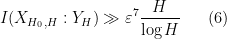
One can however still use these simpler models of Shannon entropy to be able to guess arguments that would work for general random variables. An example of this comes from my paper on the logarithmically averaged Chowla conjecture, in which I showed among other things that
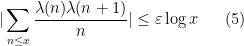
\displaystyle |\sum_{n \leq x} \frac{\lambda(n) \lambda(n+1)}{n}| \leq \varepsilon \log x \ \ \ \ \ (5)

whenever {x} was sufficiently large depending on {\varepsilon>0}, where {\lambda} is the Liouville function. The information-theoretic part of the proof was as follows. Given some intermediate scale {H} between {1} and {x}, one can form certain random variables {X_H, Y_H}. The random variable {X_H} is a sign pattern of the form {(\lambda(n+1),\dots,\lambda(n+H))} where {n} is a random number chosen from {1} to {x} (with logarithmic weighting). The random variable {Y_H} was tuple {(n \hbox{ mod } p)_{p \sim \varepsilon^2 H}} of reductions of {n} to primes {p} comparable to {\varepsilon^2 H}. Roughly speaking, what was implicitly shown in the paper (after using the multiplicativity of {\lambda}, the circle method, and the Matomaki-Radziwill theorem on short averages of multiplicative functions) is that if the inequality (5) fails, then there was a lower bound

\displaystyle I( X_H : Y_H ) \gg \varepsilon^7 \frac{H}{\log H}

on the mutual information between {X_H} and {Y_H}. From translation invariance, this also gives the more general lower bound

\displaystyle I( X_{H_0,H} : Y_H ) \gg \varepsilon^7 \frac{H}{\log H} \ \ \ \ \ (6)

for any {H_0}, where {X_{H_0,H}} denotes the shifted sign pattern {(\lambda(n+H_0+1),\dots,\lambda(n+H_0+H))}. On the other hand, one had the entropy bounds

\displaystyle H( X_{H_0,H} ), H(Y_H) \ll H

and from concatenating sign patterns one could see that {X_{H_0,H+H'}} is equivalent to the joint random variable {(X_{H_0,H}, X_{H_0+H,H'})} for any {H_0,H,H'}. Applying these facts and using an “entropy decrement” argument, I was able to obtain a contradiction once {H} was allowed to become sufficiently large compared to {\varepsilon}, but the bound was quite weak (coming ultimately from the unboundedness of {\sum_{\log H_- \leq j \leq \log H_+} \frac{1}{j \log j}} as the interval {[H_-,H_+]} of values of {H} under consideration becomes large), something of the order of {H \sim \exp\exp\exp(\varepsilon^{-7})}; the quantity {H} needs at various junctures to be less than a small power of {\log x}, so the relationship between {x} and {\varepsilon} becomes essentially quadruple exponential in nature, {x \sim \exp\exp\exp\exp(\varepsilon^{-7})}. The basic strategy was to observe that the lower bound (6) causes some slowdown in the growth rate {H(X_{kH})/kH} of the mean entropy, in that this quantity decreased by {\gg \frac{\varepsilon^7}{\log H}} as {k} increased from {1} to {\log H}, basically by dividing {X_{kH}} into {k} components {X_{jH, H}}, {j=0,\dots,k-1} and observing from (6) each of these shares a bit of common information with the same variable {Y_H}. This is relatively clear when one works in a set model, in which {Y_H} is modeled by a set {B_H} of size {O(H)}, and {X_{H_0,H}} is modeled by a set of the form

\displaystyle X_{H_0,H} = \bigcup_{H_0 < h \leq H_0+H} A_h

for various sets {A_h} of size {O(1)} (also there is some translation symmetry that maps {A_h} to a shift {A_{h+1}} while preserving all of the {B_H}).

However, on considering the set model recently, I realised that one can be a little more efficient by exploiting the fact (basically the Chinese remainder theorem) that the random variables {Y_H} are basically jointly independent as {H} ranges over dyadic values that are much smaller than {\log x}, which in the set model corresponds to the {B_H} all being disjoint. One can then establish a variant

\displaystyle I( X_{H_0,H} : Y_H | (Y_{H'})_{H' < H}) \gg \varepsilon^7 \frac{H}{\log H} \ \ \ \ \ (7)

of (6), which in the set model roughly speaking asserts that each {B_H} claims a portion of the {\bigcup_{H_0 < h \leq H_0+H} A_h} of cardinality {\gg \varepsilon^7 \frac{H}{\log H}} that is not claimed by previous choices of {B_H}. This leads to a more efficient contradiction (relying on the unboundedness of {\sum_{\log H_- \leq j \leq \log H_+} \frac{1}{j}} rather than {\sum_{\log H_- \leq j \leq \log H_+} \frac{1}{j \log j}}) that looks like it removes one order of exponential growth, thus the relationship between {x} and {\varepsilon} is now {x \sim \exp\exp\exp(\varepsilon^{-7})}. Returning to the entropy model, one can use (7) and Shannon inequalities to establish an inequality of the form

\displaystyle \frac{1}{2H} H(X_{2H} | (Y_{H'})_{H' \leq 2H}) \leq \frac{1}{H} H(X_{H} | (Y_{H'})_{H' \leq H}) - \frac{c \varepsilon^7}{\log H}

for a small constant {c>0}, which on iterating and using the boundedness of {\frac{1}{H} H(X_{H} | (Y_{H'})_{H' \leq H})} gives the claim. (A modification of this analysis, at least on the level of the back of the envelope calculation, suggests that the Matomaki-Radziwill theorem is needed only for ranges {H} greater than {\exp( (\log\log x)^{\varepsilon^{7}} )} or so, although at this range the theorem is not significantly simpler than the general case).

Let {X} and {Y} be two random variables taking values in the same (discrete) range {R}, and let {E} be some subset of {R}, which we think of as the set of “bad” outcomes for either {X} or {Y}. If {X} and {Y} have the same probability distribution, then clearly

\displaystyle  {\bf P}( X \in E ) = {\bf P}( Y \in E ).

In particular, if it is rare for {Y} to lie in {E}, then it is also rare for {X} to lie in {E}.

If {X} and {Y} do not have exactly the same probability distribution, but their probability distributions are close to each other in some sense, then we can expect to have an approximate version of the above statement. For instance, from the definition of the total variation distance {\delta(X,Y)} between two random variables (or more precisely, the total variation distance between the probability distributions of two random variables), we see that

\displaystyle  {\bf P}(Y \in E) - \delta(X,Y) \leq {\bf P}(X \in E) \leq {\bf P}(Y \in E) + \delta(X,Y) \ \ \ \ \ (1)

for any {E \subset R}. In particular, if it is rare for {Y} to lie in {E}, and {X,Y} are close in total variation, then it is also rare for {X} to lie in {E}.

A basic inequality in information theory is Pinsker’s inequality

\displaystyle  \delta(X,Y) \leq \sqrt{\frac{1}{2} D_{KL}(X||Y)}

where the Kullback-Leibler divergence {D_{KL}(X||Y)} is defined by the formula

\displaystyle  D_{KL}(X||Y) = \sum_{x \in R} {\bf P}( X=x ) \log \frac{{\bf P}(X=x)}{{\bf P}(Y=x)}.

(See this previous blog post for a proof of this inequality.) A standard application of Jensen’s inequality reveals that {D_{KL}(X||Y)} is non-negative (Gibbs’ inequality), and vanishes if and only if {X}, {Y} have the same distribution; thus one can think of {D_{KL}(X||Y)} as a measure of how close the distributions of {X} and {Y} are to each other, although one should caution that this is not a symmetric notion of distance, as {D_{KL}(X||Y) \neq D_{KL}(Y||X)} in general. Inserting Pinsker’s inequality into (1), we see for instance that

\displaystyle  {\bf P}(X \in E) \leq {\bf P}(Y \in E) + \sqrt{\frac{1}{2} D_{KL}(X||Y)}.

Thus, if {X} is close to {Y} in the Kullback-Leibler sense, and it is rare for {Y} to lie in {E}, then it is rare for {X} to lie in {E} as well.

We can specialise this inequality to the case when {Y} a uniform random variable {U} on a finite range {R} of some cardinality {N}, in which case the Kullback-Leibler divergence {D_{KL}(X||U)} simplifies to

\displaystyle  D_{KL}(X||U) = \log N - {\bf H}(X)

where

\displaystyle  {\bf H}(X) := \sum_{x \in R} {\bf P}(X=x) \log \frac{1}{{\bf P}(X=x)}

is the Shannon entropy of {X}. Again, a routine application of Jensen’s inequality shows that {{\bf H}(X) \leq \log N}, with equality if and only if {X} is uniformly distributed on {R}. The above inequality then becomes

\displaystyle  {\bf P}(X \in E) \leq {\bf P}(U \in E) + \sqrt{\frac{1}{2}(\log N - {\bf H}(X))}. \ \ \ \ \ (2)

Thus, if {E} is a small fraction of {R} (so that it is rare for {U} to lie in {E}), and the entropy of {X} is very close to the maximum possible value of {\log N}, then it is rare for {X} to lie in {E} also.

The inequality (2) is only useful when the entropy {{\bf H}(X)} is close to {\log N} in the sense that {{\bf H}(X) = \log N - O(1)}, otherwise the bound is worse than the trivial bound of {{\bf P}(X \in E) \leq 1}. In my recent paper on the Chowla and Elliott conjectures, I ended up using a variant of (2) which was still non-trivial when the entropy {{\bf H}(X)} was allowed to be smaller than {\log N - O(1)}. More precisely, I used the following simple inequality, which is implicit in the arguments of that paper but which I would like to make more explicit in this post:

Lemma 1 (Pinsker-type inequality) Let {X} be a random variable taking values in a finite range {R} of cardinality {N}, let {U} be a uniformly distributed random variable in {R}, and let {E} be a subset of {R}. Then

\displaystyle  {\bf P}(X \in E) \leq \frac{(\log N - {\bf H}(X)) + \log 2}{\log 1/{\bf P}(U \in E)}.

Proof: Consider the conditional entropy {{\bf H}(X | 1_{X \in E} )}. On the one hand, we have

\displaystyle  {\bf H}(X | 1_{X \in E} ) = {\bf H}(X, 1_{X \in E}) - {\bf H}(1_{X \in E} )

\displaystyle  = {\bf H}(X) - {\bf H}(1_{X \in E})

\displaystyle  \geq {\bf H}(X) - \log 2

by Jensen’s inequality. On the other hand, one has

\displaystyle  {\bf H}(X | 1_{X \in E} ) = {\bf P}(X \in E) {\bf H}(X | X \in E )

\displaystyle  + (1-{\bf P}(X \in E)) {\bf H}(X | X \not \in E)

\displaystyle  \leq {\bf P}(X \in E) \log |E| + (1-{\bf P}(X \in E)) \log N

\displaystyle  = \log N - {\bf P}(X \in E) \log \frac{N}{|E|}

\displaystyle  = \log N - {\bf P}(X \in E) \log \frac{1}{{\bf P}(U \in E)},

where we have again used Jensen’s inequality. Putting the two inequalities together, we obtain the claim. \Box

Remark 2 As noted in comments, this inequality can be viewed as a special case of the more general inequality

\displaystyle  {\bf P}(X \in E) \leq \frac{D(X||Y) + \log 2}{\log 1/{\bf P}(Y \in E)}

for arbitrary random variables {X,Y} taking values in the same discrete range {R}, which follows from the data processing inequality

\displaystyle  D( f(X)||f(Y)) \leq D(X|| Y)

for arbitrary functions {f}, applied to the indicator function {f = 1_E}. Indeed one has

\displaystyle  D( 1_E(X) || 1_E(Y) ) = {\bf P}(X \in E) \log \frac{{\bf P}(X \in E)}{{\bf P}(Y \in E)}

\displaystyle + {\bf P}(X \not \in E) \log \frac{{\bf P}(X \not \in E)}{{\bf P}(Y \not \in E)}

\displaystyle  \geq {\bf P}(X \in E) \log \frac{1}{{\bf P}(Y \in E)} - h( {\bf P}(X \in E) )

\displaystyle  \geq {\bf P}(X \in E) \log \frac{1}{{\bf P}(Y \in E)} - \log 2

where {h(u) := u \log \frac{1}{u} + (1-u) \log \frac{1}{1-u}} is the entropy function.

Thus, for instance, if one has

\displaystyle  {\bf H}(X) \geq \log N - o(K)

and

\displaystyle  {\bf P}(U \in E) \leq \exp( - K )

for some {K} much larger than {1} (so that {1/K = o(1)}), then

\displaystyle  {\bf P}(X \in E) = o(1).

More informally: if the entropy of {X} is somewhat close to the maximum possible value of {\log N}, and it is exponentially rare for a uniform variable to lie in {E}, then it is still somewhat rare for {X} to lie in {E}. The estimate given is close to sharp in this regime, as can be seen by calculating the entropy of a random variable {X} which is uniformly distributed inside a small set {E} with some probability {p} and uniformly distributed outside of {E} with probability {1-p}, for some parameter {0 \leq p \leq 1}.

It turns out that the above lemma combines well with concentration of measure estimates; in my paper, I used one of the simplest such estimates, namely Hoeffding’s inequality, but there are of course many other estimates of this type (see e.g. this previous blog post for some others). Roughly speaking, concentration of measure inequalities allow one to make approximations such as

\displaystyle  F(U) \approx {\bf E} F(U)

with exponentially high probability, where {U} is a uniform distribution and {F} is some reasonable function of {U}. Combining this with the above lemma, we can then obtain approximations of the form

\displaystyle  F(X) \approx {\bf E} F(U) \ \ \ \ \ (3)

with somewhat high probability, if the entropy of {X} is somewhat close to maximum. This observation, combined with an “entropy decrement argument” that allowed one to arrive at a situation in which the relevant random variable {X} did have a near-maximum entropy, is the key new idea in my recent paper; for instance, one can use the approximation (3) to obtain an approximation of the form

\displaystyle  \sum_{j=1}^H \sum_{p \in {\mathcal P}} \lambda(n+j) \lambda(n+j+p) 1_{p|n+j}

\displaystyle  \approx \sum_{j=1}^H \sum_{p \in {\mathcal P}} \frac{\lambda(n+j) \lambda(n+j+p)}{p}

for “most” choices of {n} and a suitable choice of {H} (with the latter being provided by the entropy decrement argument). The left-hand side is tied to Chowla-type sums such as {\sum_{n \leq x} \frac{\lambda(n)\lambda(n+1)}{n}} through the multiplicativity of {\lambda}, while the right-hand side, being a linear correlation involving two parameters {j,p} rather than just one, has “finite complexity” and can be treated by existing techniques such as the Hardy-Littlewood circle method. One could hope that one could similarly use approximations such as (3) in other problems in analytic number theory or combinatorics.

A handy inequality in additive combinatorics is the Plünnecke-Ruzsa inequality:

Theorem 1 (Plünnecke-Ruzsa inequality) Let {A, B_1, \ldots, B_m} be finite non-empty subsets of an additive group {G}, such that {|A+B_i| \leq K_i |A|} for all {1 \leq i \leq m} and some scalars {K_1,\ldots,K_m \geq 1}. Then there exists a subset {A'} of {A} such that {|A' + B_1 + \ldots + B_m| \leq K_1 \ldots K_m |A'|}.

The proof uses graph-theoretic techniques. Setting {A=B_1=\ldots=B_m}, we obtain a useful corollary: if {A} has small doubling in the sense that {|A+A| \leq K|A|}, then we have {|mA| \leq K^m |A|} for all {m \geq 1}, where {mA = A + \ldots + A} is the sum of {m} copies of {A}.

In a recent paper, I adapted a number of sum set estimates to the entropy setting, in which finite sets such as {A} in {G} are replaced with discrete random variables {X} taking values in {G}, and (the logarithm of) cardinality {|A|} of a set {A} is replaced by Shannon entropy {{\Bbb H}(X)} of a random variable {X}. (Throughout this note I assume all entropies to be finite.) However, at the time, I was unable to find an entropy analogue of the Plünnecke-Ruzsa inequality, because I did not know how to adapt the graph theory argument to the entropy setting.

I recently discovered, however, that buried in a classic paper of Kaimonovich and Vershik (implicitly in Proposition 1.3, to be precise) there was the following analogue of Theorem 1:

Theorem 2 (Entropy Plünnecke-Ruzsa inequality) Let {X, Y_1, \ldots, Y_m} be independent random variables of finite entropy taking values in an additive group {G}, such that {{\Bbb H}(X+Y_i) \leq {\Bbb H}(X) + \log K_i} for all {1 \leq i \leq m} and some scalars {K_1,\ldots,K_m \geq 1}. Then {{\Bbb H}(X+Y_1+\ldots+Y_m) \leq {\Bbb H}(X) + \log K_1 \ldots K_m}.

In fact Theorem 2 is a bit “better” than Theorem 1 in the sense that Theorem 1 needed to refine the original set {A} to a subset {A'}, but no such refinement is needed in Theorem 2. One corollary of Theorem 2 is that if {{\Bbb H}(X_1+X_2) \leq {\Bbb H}(X) + \log K}, then {{\Bbb H}(X_1+\ldots+X_m) \leq {\Bbb H}(X) + (m-1) \log K} for all {m \geq 1}, where {X_1,\ldots,X_m} are independent copies of {X}; this improves slightly over the analogous combinatorial inequality. Indeed, the function {m \mapsto {\Bbb H}(X_1+\ldots+X_m)} is concave (this can be seen by using the {m=2} version of Theorem 2 (or (2) below) to show that the quantity {{\Bbb H}(X_1+\ldots+X_{m+1})-{\Bbb H}(X_1+\ldots+X_m)} is decreasing in {m}).

Theorem 2 is actually a quick consequence of the submodularity inequality

\displaystyle  {\Bbb H}(W) + {\Bbb H}(X) \leq {\Bbb H}(Y) + {\Bbb H}(Z) \ \ \ \ \ (1)

in information theory, which is valid whenever {X,Y,Z,W} are discrete random variables such that {Y} and {Z} each determine {X} (i.e. {X} is a function of {Y}, and also a function of {Z}), and {Y} and {Z} jointly determine {W} (i.e {W} is a function of {Y} and {Z}). To apply this, let {X, Y, Z} be independent discrete random variables taking values in {G}. Observe that the pairs {(X,Y+Z)} and {(X+Y,Z)} each determine {X+Y+Z}, and jointly determine {(X,Y,Z)}. Applying (1) we conclude that

\displaystyle  {\Bbb H}(X,Y,Z) + {\Bbb H}(X+Y+Z) \leq {\Bbb H}(X,Y+Z) + {\Bbb H}(X+Y,Z)

which after using the independence of {X,Y,Z} simplifies to the sumset submodularity inequality

\displaystyle  {\Bbb H}(X+Y+Z) + {\Bbb H}(Y) \leq {\Bbb H}(X+Y) + {\Bbb H}(Y+Z) \ \ \ \ \ (2)

(this inequality was also recently observed by Madiman; it is the {m=2} case of Theorem 2). As a corollary of this inequality, we see that if {{\Bbb H}(X+Y_i) \leq {\Bbb H}(X) + \log K_i}, then

\displaystyle  {\Bbb H}(X+Y_1+\ldots+Y_i) \leq {\Bbb H}(X+Y_1+\ldots+Y_{i-1}) + \log K_i,

and Theorem 2 follows by telescoping series.

The proof of Theorem 2 seems to be genuinely different from the graph-theoretic proof of Theorem 1. It would be interesting to see if the above argument can be somehow adapted to give a stronger version of Theorem 1. Note also that both Theorem 1 and Theorem 2 have extensions to more general combinations of {X,Y_1,\ldots,Y_m} than {X+Y_i}; see this paper and this paper respectively.

Read the rest of this entry »

I am posting here four more of my Mahler lectures, each of which is based on earlier talks of mine:

As always, comments, corrections, and other feedback are welcome.

There are many situations in combinatorics in which one is running some sort of iteration algorithm to continually “improve” some object {A}; each loop of the algorithm replaces {A} with some better version {A'} of itself, until some desired property of {A} is attained and the algorithm halts. In order for such arguments to yield a useful conclusion, it is often necessary that the algorithm halts in a finite amount of time, or (even better), in a bounded amount of time. (In general, one cannot use infinitary iteration tools, such as transfinite induction or Zorn’s lemma, in combinatorial settings, because the iteration processes used to improve some target object {A} often degrade some other finitary quantity {B} in the process, and an infinite iteration would then have the undesirable effect of making {B} infinite.)

A basic strategy to ensure termination of an algorithm is to exploit a monotonicity property, or more precisely to show that some key quantity keeps increasing (or keeps decreasing) with each loop of the algorithm, while simultaneously staying bounded. (Or, as the economist Herbert Stein was fond of saying, “If something cannot go on forever, it must stop.”)

Here are four common flavours of this monotonicity strategy:

  • The mass increment argument. This is perhaps the most familiar way to ensure termination: make each improved object {A'} “heavier” than the previous one {A} by some non-trivial amount (e.g. by ensuring that the cardinality of {A'} is strictly greater than that of {A}, thus {|A'| \geq |A|+1}). Dually, one can try to force the amount of “mass” remaining “outside” of {A} in some sense to decrease at every stage of the iteration. If there is a good upper bound on the “mass” of {A} that stays essentially fixed throughout the iteration process, and a lower bound on the mass increment at each stage, then the argument terminates. Many “greedy algorithm” arguments are of this type. The proof of the Hahn decomposition theorem in measure theory also falls into this category. The general strategy here is to keep looking for useful pieces of mass outside of {A}, and add them to {A} to form {A'}, thus exploiting the additivity properties of mass. Eventually no further usable mass remains to be added (i.e. {A} is maximal in some {L^1} sense), and this should force some desirable property on {A}.
  • The density increment argument. This is a variant of the mass increment argument, in which one increments the “density” of {A} rather than the “mass”. For instance, {A} might be contained in some ambient space {P}, and one seeks to improve {A} to {A'} (and {P} to {P'}) in such a way that the density of the new object in the new ambient space is better than that of the previous object (e.g. {|A'|/|P'| \geq |A|/|P| + c} for some {c>0}). On the other hand, the density of {A} is clearly bounded above by {1}. As long as one has a sufficiently good lower bound on the density increment at each stage, one can conclude an upper bound on the number of iterations in the algorithm. The prototypical example of this is Roth’s proof of his theorem that every set of integers of positive upper density contains an arithmetic progression of length three. The general strategy here is to keep looking for useful density fluctuations inside {A}, and then “zoom in” to a region of increased density by reducing {A} and {P} appropriately. Eventually no further usable density fluctuation remains (i.e. {A} is uniformly distributed), and this should force some desirable property on {A}.
  • The energy increment argument. This is an “{L^2}” analogue of the “{L^1}“-based mass increment argument (or the “{L^\infty}“-based density increment argument), in which one seeks to increments the amount of “energy” that {A} captures from some reference object {X}, or (equivalently) to decrement the amount of energy of {X} which is still “orthogonal” to {A}. Here {A} and {X} are related somehow to a Hilbert space, and the energy involves the norm on that space. A classic example of this type of argument is the existence of orthogonal projections onto closed subspaces of a Hilbert space; this leads among other things to the construction of conditional expectation in measure theory, which then underlies a number of arguments in ergodic theory, as discussed for instance in this earlier blog post. Another basic example is the standard proof of the Szemerédi regularity lemma (where the “energy” is often referred to as the “index”). These examples are related; see this blog post for further discussion. The general strategy here is to keep looking for useful pieces of energy orthogonal to {A}, and add them to {A} to form {A'}, thus exploiting square-additivity properties of energy, such as Pythagoras’ theorem. Eventually, no further usable energy outside of {A} remains to be added (i.e. {A} is maximal in some {L^2} sense), and this should force some desirable property on {A}.
  • The rank reduction argument. Here, one seeks to make each new object {A'} to have a lower “rank”, “dimension”, or “order” than the previous one. A classic example here is the proof of the linear algebra fact that given any finite set of vectors, there exists a linearly independent subset which spans the same subspace; the proof of the more general Steinitz exchange lemma is in the same spirit. The general strategy here is to keep looking for “collisions” or “dependencies” within {A}, and use them to collapse {A} to an object {A'} of lower rank. Eventually, no further usable collisions within {A} remain, and this should force some desirable property on {A}.

Much of my own work in additive combinatorics relies heavily on at least one of these types of arguments (and, in some cases, on a nested combination of two or more of them). Many arguments in nonlinear partial differential equations also have a similar flavour, relying on various monotonicity formulae for solutions to such equations, though the objective in PDE is usually slightly different, in that one wants to keep control of a solution as one approaches a singularity (or as some time or space coordinate goes off to infinity), rather than to ensure termination of an algorithm. (On the other hand, many arguments in the theory of concentration compactness, which is used heavily in PDE, does have the same algorithm-terminating flavour as the combinatorial arguments; see this earlier blog post for more discussion.)

Recently, a new species of monotonicity argument was introduced by Moser, as the primary tool in his elegant new proof of the Lovász local lemma. This argument could be dubbed an entropy compression argument, and only applies to probabilistic algorithms which require a certain collection {R} of random “bits” or other random choices as part of the input, thus each loop of the algorithm takes an object {A} (which may also have been generated randomly) and some portion of the random string {R} to (deterministically) create a better object {A'} (and a shorter random string {R'}, formed by throwing away those bits of {R} that were used in the loop). The key point is to design the algorithm to be partially reversible, in the sense that given {A'} and {R'} and some additional data {H'} that logs the cumulative history of the algorithm up to this point, one can reconstruct {A} together with the remaining portion {R} not already contained in {R'}. Thus, each stage of the argument compresses the information-theoretic content of the string {A+R} into the string {A'+R'+H'} in a lossless fashion. However, a random variable such as {A+R} cannot be compressed losslessly into a string of expected size smaller than the Shannon entropy of that variable. Thus, if one has a good lower bound on the entropy of {A+R}, and if the length of {A'+R'+H'} is significantly less than that of {A+R} (i.e. we need the marginal growth in the length of the history file {H'} per iteration to be less than the marginal amount of randomness used per iteration), then there is a limit as to how many times the algorithm can be run, much as there is a limit as to how many times a random data file can be compressed before no further length reduction occurs.

It is interesting to compare this method with the ones discussed earlier. In the previous methods, the failure of the algorithm to halt led to a new iteration of the object {A} which was “heavier”, “denser”, captured more “energy”, or “lower rank” than the previous instance of {A}. Here, the failure of the algorithm to halt leads to new information that can be used to “compress” {A} (or more precisely, the full state {A+R}) into a smaller amount of space. I don’t know yet of any application of this new type of termination strategy to the fields I work in, but one could imagine that it could eventually be of use (perhaps to show that solutions to PDE with sufficiently “random” initial data can avoid singularity formation?), so I thought I would discuss it here.

Below the fold I give a special case of Moser’s argument, based on a blog post of Lance Fortnow on this topic.

Read the rest of this entry »

The most fundamental unsolved problem in complexity theory is undoubtedly the P=NP problem, which asks (roughly speaking) whether a problem which can be solved by a non-deterministic polynomial-time (NP) algorithm, can also be solved by a deterministic polynomial-time (P) algorithm. The general belief is that {P \neq NP}, i.e. there exist problems which can be solved by non-deterministic polynomial-time algorithms but not by deterministic polynomial-time algorithms.

One reason why the {P \neq NP} question is so difficult to resolve is that a certain generalisation of this question has an affirmative answer in some cases, and a negative answer in other cases. More precisely, if we give all the algorithms access to an oracle, then for one choice {A} of this oracle, all the problems that are solvable by non-deterministic polynomial-time algorithms that calls {A} ({NP^A}), can also be solved by a deterministic polynomial-time algorithm algorithm that calls {A} ({P^A}), thus {P^A = NP^A}; but for another choice {B} of this oracle, there exist problems solvable by non-deterministic polynomial-time algorithms that call {B}, which cannot be solved by a deterministic polynomial-time algorithm that calls {B}, thus {P^B \neq NP^B}. One particular consequence of this result (which is due to Baker, Gill, and Solovay) is that there cannot be any relativisable proof of either {P=NP} or {P \neq NP}, where “relativisable” means that the proof would also work without any changes in the presence of an oracle.

The Baker-Gill-Solovay result was quite surprising, but the idea of the proof turns out to be rather simple. To get an oracle {A} such that {P^A=NP^A}, one basically sets {A} to be a powerful simulator that can simulate non-deterministic machines (and, furthermore, can also simulate itself); it turns out that any PSPACE-complete oracle would suffice for this task. To get an oracle {B} for which {P^B \neq NP^B}, one has to be a bit sneakier, setting {B} to be a query device for a sparse set of random (or high-complexity) strings, which are too complex to be guessed at by any deterministic polynomial-time algorithm.

Unfortunately, the simple idea of the proof can be obscured by various technical details (e.g. using Turing machines to define {P} and {NP} precisely), which require a certain amount of time to properly absorb. To help myself try to understand this result better, I have decided to give a sort of “allegory” of the proof, based around a (rather contrived) story about various students trying to pass a multiple choice test, which avoids all the technical details but still conveys the basic ideas of the argument. This allegory was primarily for my own benefit, but I thought it might also be of interest to some readers here (and also has some tangential relation to the proto-polymath project of determinstically finding primes), so I reproduce it below.

Read the rest of this entry »

[This post should have appeared several months ago, but I didn’t have a link to the newsletter at the time, and I subsequently forgot about it until now.  -T.]

Last year, Emmanuel Candés and I were two of the recipients of the 2008 IEEE Information Theory Society Paper Award, for our paper “Near-optimal signal recovery from random projections: universal encoding strategies?” published in IEEE Inf. Thy..  (The other recipient is David Donoho, for the closely related paper “Compressed sensing” in the same journal.)  These papers helped initiate the modern subject of compressed sensing, which I have talked about earlier on this blog, although of course they also built upon a number of important precursor results in signal recovery, high-dimensional geometry, Fourier analysis, linear programming, and probability.  As part of our response to this award, Emmanuel and I wrote a short piece commenting on these developments, entitled “Reflections on compressed sensing“, which appears in the Dec 2008 issue of the IEEE Information Theory newsletter.  In it we place our results in the context of these precursor results, and also mention some of the many active directions (theoretical, numerical, and applied) that compressed sensing is now developing in.

Archives