
You are currently browsing the category archive for the ‘254A – analytic prime number theory’ category.
Let us call an arithmetic function 


- The Möbius function
;
- The Liouville function
;
- “Archimedean” characters
(which I call Archimedean because they are pullbacks of a Fourier character
on the multiplicative group
, which has the Archimedean property);
- Dirichlet characters (or “non-Archimedean” characters)
(which are essentially pullbacks of Fourier characters on a multiplicative cyclic group
with the discrete (non-Archimedean) metric);
- Hybrid characters
.
The space of
Given a multiplicative function 

for large values of 
where 


as 
Exercise 1 Without using the prime number theorem, show that (1) is also equivalent to
as
and
.)
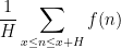
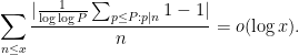
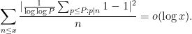
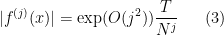
Henceforth we shall focus our discussion more on the Liouville function, and turn our attention to averages on shorter intervals. From (2) one has

as 


The situation is better when one asks to understand the mean value on almost all short intervals, rather than all intervals. There are several equivalent ways to formulate this question:
Exercise 2 Let
be a function of
and
as
- (i) One has
as
outside of a set of measure
.
- (ii) One has
as
- (iii) One has
as


As it turns out the second moment formulation in (iii) will be the most convenient for us to work with in this set of notes, as it is well suited to Fourier-analytic techniques (and in particular the Plancherel theorem).
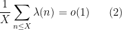
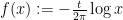
Using zero density methods, for instance, it was shown by Ramachandra that

whenever 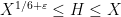


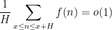
Theorem 3 (Matomaki-Radziwill theorem for Liouville) For any
, one has
for some absolute constant
.
In fact they prove a slightly more precise result: see Theorem 1 of that paper. In particular, they obtain the asymptotic (4) for any function
Exercise 4 In this exercise you may use Theorem 3 freely.
- (i) Establish the upper bound
for some absolute constant
would hold for almost all
; use this to create many intervals
for which
is extremely large.)
- (ii) Show that Theorem 3 also holds with
replaced by
, where
is the principal character of period
. (Use the fact that
for all
to (i).
(There is a curious asymmetry to the difficulty level of these bounds; the upper bound in (ii) was established much earlier by Harman, Pintz, and Wolke, but the lower bound in (i) was only established in the Matomaki-Radziwill paper.)


The techniques discussed previously were highly complex-analytic in nature, relying in particular on the fact that functions such as 


Definition 5 (Pretentious distance) Given two
, the pretentious distance
between

Note that one can also define an infinite version 


Proposition 6 (Logarithmically averaged version of Halasz) Let
for an absolute constant

In particular, if 
If one works with non-logarithmic averages 


Theorem 7 (Halasz’s theorem) Let
for an absolute constant
.
Informally, we refer to a 


In the contrapositive, Halasz’ theorem can be formulated as the assertion that if one has a large mean
for some 

for some 
Among other things, Halasz’s theorem gives yet another proof of the prime number theorem (1); see Section 2.
We now give a version of the Matomaki-Radziwill theorem for general (non-pretentious) multiplicative functions that is formulated in a similar contrapositive (or “inverse theorem”) fashion, though to simplify the presentation we only state a qualitative version that does not give explicit bounds.
Theorem 8 ((Qualitative) Matomaki-Radziwill theorem) Let
, and let
, with
. Suppose that
Then one has
for some
.


The condition
Exercise 9 Let
. Let
. Show that

Combining Theorem 8 with standard non-pretentiousness facts about the Liouville function (see Exercise 24), we recover Theorem 3 (but with a decay rate of only 
With our current state of knowledge, the only arguments that can establish the full strength of Halasz and Matomaki-Radziwill theorems are Fourier analytic in nature, relating sums involving an arithmetic function
which one can view as a discrete Fourier transform of 

Proposition 10 (Parseval type identity) Let
be finitely supported arithmetic functions, and let
be a Schwartz function. Then
where
is the Fourier transform of
. (Note that the finite support of
ensure that both sides of the identity are absolutely convergent.)

The restriction that
Proof: By expanding out the Dirichlet series, it suffices to show that
for any natural numbers 

For applications to Halasz type theorems, one sets 


Exercise 11 (Plancherel type identity) If
is a Schwartz function, establish the identity

In contrast, information about the non-pretentious nature of a multiplicative function 

It will be convenient to formalise the notion of
Definition 12 (Fourier norms) Let
be a bounded measurable set. We define the Fourier
the Fourier
and the Fourier

One could more generally define 


As mentioned above, Halasz’s theorem gives good control on the Fourier
Exercise 13 (Fourier
be an interval in
for some
, let
, and let
(Hint: you will need to use summation by parts (or an equivalent device) to deal with a
weight.)

Meanwhile, the Plancherel identity in Exercise 11 gives good control on the Fourier
Exercise 14 (
, and let
Conclude in particular that if
for some
and
, then
![\displaystyle \| f \|_{FL^2([-T,T])}^2 \ll \sum_n \frac{1}{n} (\frac{T}{n} \sum_{m: |n-m| \leq n/T} |f(m)|)^2.](https://s0.wp.com/latex.php?latex=%5Cdisplaystyle+%5C%7C+f+%5C%7C_%7BFL%5E2%28%5B-T%2CT%5D%29%7D%5E2+%5Cll+%5Csum_n+%5Cfrac%7B1%7D%7Bn%7D+%28%5Cfrac%7BT%7D%7Bn%7D+%5Csum_%7Bm%3A+%7Cn-m%7C+%5Cleq+n%2FT%7D+%7Cf%28m%29%7C%29%5E2.&bg=ffffff&fg=000000&s=0&c=20201002)
![\displaystyle \| f \|_{FL^2([-T,T])}^2 \ll C^{O(1)} \frac{1}{N} \sum_n |f(n)|^2.](https://s0.wp.com/latex.php?latex=%5Cdisplaystyle+%5C%7C+f+%5C%7C_%7BFL%5E2%28%5B-T%2CT%5D%29%7D%5E2+%5Cll+C%5E%7BO%281%29%7D+%5Cfrac%7B1%7D%7BN%7D+%5Csum_n+%7Cf%28n%29%7C%5E2.&bg=ffffff&fg=000000&s=0&c=20201002)
In the simplest case of the logarithmically averaged Halasz theorem (Proposition 6), Fourier


The strategy is then to factor (or approximately factor) the original function 


![{[-T,T]}](https://s0.wp.com/latex.php?latex=%7B%5B-T%2CT%5D%7D&bg=ffffff&fg=000000&s=0&c=20201002)
There are several ways to achieve the desired factorisation. In the case of Halasz’s theorem, we can simply work with a crude version of the Euler product factorisation, dividing the primes into three categories (“small”, “medium”, and “large” primes) and expressing ![{[P,Q]}](https://s0.wp.com/latex.php?latex=%7B%5BP%2CQ%5D%7D&bg=ffffff&fg=000000&s=0&c=20201002)

![\displaystyle w_{[P,Q]}(n) = \frac{1}{\log\log Q - \log\log P} \sum_{P \leq p \leq Q} 1_{n=p} \ \ \ \ \ (7)](https://s0.wp.com/latex.php?latex=%5Cdisplaystyle+w_%7B%5BP%2CQ%5D%7D%28n%29+%3D+%5Cfrac%7B1%7D%7B%5Clog%5Clog+Q+-+%5Clog%5Clog+P%7D+%5Csum_%7BP+%5Cleq+p+%5Cleq+Q%7D+1_%7Bn%3Dp%7D+%5C+%5C+%5C+%5C+%5C+%287%29&bg=ffffff&fg=000000&s=0&c=20201002)
then we have
![\displaystyle 1 \approx 1 * w_{[P,Q]}](https://s0.wp.com/latex.php?latex=%5Cdisplaystyle+1+%5Capprox+1+%2A+w_%7B%5BP%2CQ%5D%7D&bg=ffffff&fg=000000&s=0&c=20201002)
and more generally we have a twisted approximation
![\displaystyle f \approx f * fw_{[P,Q]}](https://s0.wp.com/latex.php?latex=%5Cdisplaystyle+f+%5Capprox+f+%2A+fw_%7B%5BP%2CQ%5D%7D&bg=ffffff&fg=000000&s=0&c=20201002)
for multiplicative functions ![{f w_{[P,Q]}}](https://s0.wp.com/latex.php?latex=%7Bf+w_%7B%5BP%2CQ%5D%7D%7D&bg=ffffff&fg=000000&s=0&c=20201002)
Read the rest of this entry »
In these notes we presume familiarity with the basic concepts of probability theory, such as random variables (which could take values in the reals, vectors, or other measurable spaces), probability, and expectation. Much of this theory is in turn based on measure theory, which we will also presume familiarity with. See for instance this previous set of lecture notes for a brief review.
The basic objects of study in analytic number theory are deterministic; there is nothing inherently random about the set of prime numbers, for instance. Despite this, one can still interpret many of the averages encountered in analytic number theory in probabilistic terms, by introducing random variables into the subject. Consider for instance the form

of the prime number theorem (where we take the limit

where 

After dividing by

With probabilistic intuition, one may expect the random variables 


which by (2) is equal to
The asymptotic (3) is widely believed (it is a special case of the Chowla conjecture, which we will discuss in later notes; while there has been recent progress towards establishing it rigorously, it remains open for now.
How would one try to make these probabilistic intuitions more rigorous? The first thing one needs to do is find a more quantitative measurement of what it means for two random variables to be “approximately” independent. There are several candidates for such measurements, but we will focus in these notes on two particularly convenient measures of approximate independence: the “

of (3), which is implied by (3) but strictly weaker (much as the prime number theorem (1) implies the bound 
As with many other situations in analytic number theory, we can exploit the fact that certain assertions (such as approximate independence) can become significantly easier to prove if one only seeks to establish them on average, rather than uniformly. For instance, given two random variables 


In the fall quarter (starting Sep 27) I will be teaching a graduate course on analytic prime number theory. This will be similar to a graduate course I taught in 2015, and in particular will reuse several of the lecture notes from that course, though it will also incorporate some new material (and omit some material covered in the previous course, to compensate). I anticipate covering the following topics:
- Elementary multiplicative number theory
- Complex-analytic multiplicative number theory
- The entropy decrement argument
- Bounds for exponential sums
- Zero density theorems
- Halasz’s theorem and the Matomaki-Radziwill theorem
- The circle method
- (If time permits) Chowla’s conjecture and the Erdos discrepancy problem [Update: I did not end up writing notes on this topic.]
Lecture notes for topics 3, 6, and 8 will be forthcoming.
We have seen in previous notes that the operation of forming a Dirichlet series
or twisted Dirichlet series

is an incredibly useful tool for questions in multiplicative number theory. Such series can be viewed as a multiplicative Fourier transform, since the functions 

Similarly, it turns out that the operation of forming an additive Fourier series

where 


- (Even Goldbach conjecture) Is it true that every even natural number
greater than two can be expressed as the sum
of two primes?
- (Odd Goldbach conjecture) Is it true that every odd natural number
of three primes?
- (Waring problem) For each natural number
, what is the least natural number
such that every natural number
powers?
- (Asymptotic Waring problem) For each natural number
such that every sufficiently large natural number
- (Partition function problem) For any natural number
denote the number of representations of
where
are natural numbers. What is the asymptotic behaviour of
?
The Waring problem and its asymptotic version will not be discussed further here, save to note that the Vinogradov mean value theorem (Theorem 13 from Notes 5) and its variants are particularly useful for getting good bounds on
Instead, we will focus our attention on the odd Goldbach conjecture as our model problem. (The even Goldbach conjecture, which involves only two variables instead of three, is unfortunately not amenable to a circle method approach for a variety of reasons, unless the statement is replaced with something weaker, such as an averaged statement; see this previous blog post for further discussion. On the other hand, the methods here can obtain weaker versions of the even Goldbach conjecture, such as showing that “almost all” even numbers are the sum of two primes; see Exercise 34 below.) In particular, we will establish the following celebrated theorem of Vinogradov:
Theorem 1 (Vinogradov’s theorem) Every sufficiently large odd number
Recently, the restriction that 
We will in fact show the more precise statement:
Theorem 2 (Quantitative Vinogradov theorem) Let
be an natural number. Then
The implied constants are ineffective.

We dropped the hypothesis that 
Unfortunately, due to the ineffectivity of the constants in Theorem 2 (a consequence of the reliance on the Siegel-Walfisz theorem in the proof of that theorem), one cannot quantify explicitly what “sufficiently large” means in Theorem 1 directly from Theorem 2. However, there is a modification of this theorem which gives effective bounds; see Exercise 32 below.
Exercise 4 Obtain a heuristic derivation of the main term
using the modified Cramér model (Section 1 of Supplement 4).
To prove Theorem 2, we consider the more general problem of estimating sums of the form

for various integers 
Suppose that 


A basic observation is that this upper bound is attainable if 


as
The key to the success of the circle method lies in the converse of the above statement: the only way that the trivial upper bound (2) comes close to being sharp is when 
Exercise 5 Let
and

The traditional approach to using the circle method to compute sums such as 


This traditional approach is covered in many places, such as this text of Vaughan. We will emphasise in this set of notes a slightly different perspective on the circle method, coming from recent developments in additive combinatorics; this approach does not quite give the sharpest quantitative estimates, but it allows for easier generalisation to more combinatorial contexts, for instance when replacing the primes by dense subsets of the primes, or replacing the equation
From Exercise 5 and Hölder’s inequality, we immediately obtain
Corollary 6 Let
Similarly for permutations of the

In the case when ![{[1,N]}](https://s0.wp.com/latex.php?latex=%7B%5B1%2CN%5D%7D&bg=ffffff&fg=000000&s=0&c=20201002)


Thus, one possible strategy for estimating the sum 


Exercise 7 Let
be a random subset of
has an independent probability of
of lying in
- (i) If
and
, show that with probability
as
uniformly in
) using a concentration of measure inequality, such as Hoeffding’s inequality. To obtain the uniformity in
and apply the union bound).
- (ii) Show that with probability
representations of the form
with
(with
treated as an ordered triple, rather than an unordered one).
In the case when 


uniformly in 
This suggests a strategy for proving Vinogradov’s theorem: find an approximant 

and obtain an approximation by truncating 

Thus, for instance, if

One could also use the slightly smoother approximation

in which case we would take
The function 

Theorem 8 (Davenport’s estimate) For any
and
, we have
uniformly for all

This estimate will be proven by splitting into two cases. In the “major arc” case when 


A somewhat different looking approximation for the von Mangoldt function that also turns out to be quite useful is
for some 
The approximation (8) can be written in a way that makes it more similar to (7):
Exercise 9 Show that the right-hand side of (8) can be rewritten as
where
Then, show the inequalities
and conclude that
(Hint: for the latter estimate, use Theorem 27 of Notes 1.)


The coefficients 
Another approximation to
where 


for 


Exercise 10 With
for all natural numbers

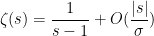
A major topic of interest of analytic number theory is the asymptotic behaviour of the Riemann zeta function 


![{\log |\zeta|: {\bf C} \rightarrow [-\infty,+\infty]}](https://s0.wp.com/latex.php?latex=%7B%5Clog+%7C%5Czeta%7C%3A+%7B%5Cbf+C%7D+%5Crightarrow+%5B-%5Cinfty%2C%2B%5Cinfty%5D%7D&bg=ffffff&fg=000000&s=0&c=20201002)


One has the classical estimate
 and
and  (say), so that
(See e.g. Exercise 37 from Supplement 3.) In view of this, let us define the normalised log-magnitudes ![{F_T: {\bf C} \rightarrow [-\infty,+\infty]}](https://s0.wp.com/latex.php?latex=%7BF_T%3A+%7B%5Cbf+C%7D+%5Crightarrow+%5B-%5Cinfty%2C%2B%5Cinfty%5D%7D&bg=ffffff&fg=000000&s=0&c=20201002)

informally, this is a normalised window into 

- (i) The bound (1) implies that
, thus for any compact set
we have
for
and
sufficiently large. In fact the implied constant in
only depends on the projection of
- (ii) For
, we have the bounds
which implies that
to zero in the region
.
- (iii) The functional equation, together with the symmetry
, implies that
which by Exercise 17 of Supplement 3 shows that
as
. In particular, when combined with the previous item, we see that
converges locally uniformly as
in the region
.
- (iv) From Jensen’s formula (Theorem 16 of Supplement 2) we see that
is a subharmonic function, and thus
for any disk
, where the integral is with respect to area measure. From this and (ii) we conclude that
for any disk with
and sufficiently large
for sufficiently large


From (iv) and the usual Arzela-Ascoli diagonalisation argument, we see that the 


- (i)
.
- (ii)
.
- (iii) We have the functional equation
for all
for
.
- (iv)
Unfortunately, (i)-(iv) fail to characterise 


We pause to address one minor technicality. We have defined 
for any 


By a classical theorem of Riesz, a function 


away from the real axis, where 


where 

Thus
Using this machinery, we can recover many classical theorems about the Riemann zeta function by “soft” arguments that do not require extensive calculation. Here are some examples:
Theorem 1 The Riemann hypothesis implies the Lindelöf hypothesis.
Proof: It suffices to show that any limiting profile 

In fact, we have the following sharper statement:
Theorem 2 (Backlund) The Lindelöf hypothesis is equivalent to the assertion that for any fixed
, the number of zeroes in the region
is
as
Proof: If the latter claim holds, then for any 


Conversely, suppose the claim fails, then we can find a sequence 


Theorem 3 (Littlewood) Assume the Lindelöf hypothesis. Then for any fixed
, the number of zeroes in the region
is
as
Proof: By the previous arguments, the only possible normalised limiting profile for 


Even without the Lindelöf hypothesis, we have the following result:
Theorem 4 (Titchmarsh) For any fixed
zeroes in the region
Among other things, this theorem recovers a classical result of Littlewood that the gaps between the imaginary parts of the zeroes goes to zero, even without assuming unproven conjectures such as the Riemann or Lindelöf hypotheses.
Proof: Suppose for contradiction that this were not the case, then we can find 


Exercise 5 Use limiting profiles to obtain the matching upper bound of
for the number of zeroes in
Remark 6 One can remove the need to take limiting profiles in the above arguments if one can come up with quantitative (or “hard”) substitutes for qualitative (or “soft”) results such as the unique continuation property for harmonic functions. This would also allow one to replace the qualitative decay rates
or
. Indeed, the classical proofs of the above theorems come with quantitative bounds that are typically of this form (see e.g. the text of Titchmarsh for details).
Exercise 7 Let
denote the quantity
, where the branch of the argument is taken by using a line segment connecting
to (say)
, and then to
for
converges in the sense of distributions to the function
, or equivalently
Conclude in particular that if the Lindelöf hypothesis holds, then
as

A little bit more about the normalised limit profiles 


Better control on limiting profiles is available if we do not insist on controlling
In analytic number theory, it is a well-known phenomenon that for many arithmetic functions

than it is to estimate summatory functions such as

(Here we are normalising 


Viewed conversely, whenever one has a difficult estimate on a summatory function such as 
We begin with Halasz’s theorem. Here is a version of this theorem, due to Montgomery and to Tenenbaum:
Theorem 1 (Halasz-Montgomery-Tenenbaum) Let
and
Then one has

Informally, this theorem asserts that 


Theorem 2 (Cheap Halasz) Let

Note that now that we are content with estimating exponential sums, we no longer need to preclude the possibility that 

To prove this theorem, we first need a special case of the Turan-Kubilius inequality.
Lemma 3 (Turan-Kubilius) Let
be a quantity depending on
and
as
Informally, this lemma is asserting that

for most large numbers
![\displaystyle 1 \approx 1 * \frac{1}{\log\log P} 1_{{\mathcal P} \cap [1,P]}.](https://s0.wp.com/latex.php?latex=%5Cdisplaystyle+1+%5Capprox+1+%2A+%5Cfrac%7B1%7D%7B%5Clog%5Clog+P%7D+1_%7B%7B%5Cmathcal+P%7D+%5Ccap+%5B1%2CP%5D%7D.&bg=ffffff&fg=000000&s=0&c=20201002)
This type of estimate was previously discussed as a tool to establish a criterion of Katai and Bourgain-Sarnak-Ziegler for Möbius orthogonality estimates in this previous blog post. See also Section 5 of Notes 1 for some similar computations.
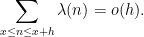
Proof: By Cauchy-Schwarz it suffices to show that
Expanding out the square, it suffices to show that

for 
We just show the 

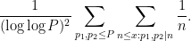
We can estimate the inner sum as ![{(1+o(1)) \frac{1}{[p_1,p_2]} \log x}](https://s0.wp.com/latex.php?latex=%7B%281%2Bo%281%29%29+%5Cfrac%7B1%7D%7B%5Bp_1%2Cp_2%5D%7D+%5Clog+x%7D&bg=ffffff&fg=000000&s=0&c=20201002)

![\displaystyle \sum_{p_1, p_2 \leq P} \frac{1}{[p_1,p_2]} = (1+o(1)) (\log\log P)^2](https://s0.wp.com/latex.php?latex=%5Cdisplaystyle+%5Csum_%7Bp_1%2C+p_2+%5Cleq+P%7D+%5Cfrac%7B1%7D%7B%5Bp_1%2Cp_2%5D%7D+%3D+%281%2Bo%281%29%29+%28%5Clog%5Clog+P%29%5E2&bg=ffffff&fg=000000&s=0&c=20201002)
and the claim follows.
Remark 4 As an alternative to the Turan-Kubilius inequality, one can use the Ramaré identity
(see e.g. Section 17.3 of Friedlander-Iwaniec). This identity turns out to give superior quantitative results than the Turan-Kubilius inequality in applications; see the paper of Matomaki and Radziwiłł for an instance of this.
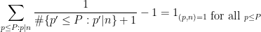
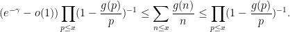
We now prove Theorem 2. Let 

We rearrange the left-hand side as

We now replace the constraint 


which by Mertens’ theorem is 
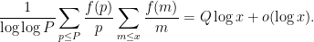
But by definition of 
![\displaystyle [1 - \frac{1}{\log\log P} \sum_{p \leq P} \frac{f(p)}{p}] Q = o(1). \ \ \ \ \ (3)](https://s0.wp.com/latex.php?latex=%5Cdisplaystyle+%5B1+-+%5Cfrac%7B1%7D%7B%5Clog%5Clog+P%7D+%5Csum_%7Bp+%5Cleq+P%7D+%5Cfrac%7Bf%28p%29%7D%7Bp%7D%5D+Q+%3D+o%281%29.+%5C+%5C+%5C+%5C+%5C+%283%29&bg=ffffff&fg=000000&s=0&c=20201002)
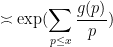
From Mertens’ theorem, the expression in brackets can be rewritten as

and so the real part of this expression is

By (1), Mertens’ theorem and the hypothesis on

for any 

and thus the expression in brackets has real part 
The Turan-Kubilius argument is certainly not the most efficient way to estimate sums such as 
Exercise 5 (Granville-Koukoulopoulos-Matomaki)
- (i) If
for all primes
as
, where
is the completely multiplicative function with
for all primes
- (ii) If
, show that
for all
.

Now we turn to a very recent result of Matomaki and Radziwiłł on mean values of multiplicative functions in short intervals. For sake of illustration we specialise their results to the simpler case of the Liouville function
Theorem 6 (Matomaki-Radziwiłł, special case) Let
be a quantity going to infinity as

A simple sieving argument (see Exercise 18 of Supplement 4) shows that one can replace
Of course, (4) improves upon the trivial bound of 


as 
Below the fold, we give a “cheap” version of the Matomaki-Radziwiłł argument. More precisely, we establish
Theorem 7 (Cheap Matomaki-Radziwiłł) Let
. Then

 .
.Note that (5) improves upon the trivial bound of 
In the previous set of notes, we saw how zero-density theorems for the Riemann zeta function, when combined with the zero-free region of Vinogradov and Korobov, could be used to obtain prime number theorems in short intervals. It turns out that a more sophisticated version of this type of argument also works to obtain prime number theorems in arithmetic progressions, in particular establishing the celebrated theorem of Linnik:
Theorem 1 (Linnik’s theorem) Let
be a primitive residue class. Then
.
In fact it is known that one can find a prime 

We will not aim to obtain the optimal exponents for Linnik’s theorem here, and follow the treatment in Chapter 18 of Iwaniec and Kowalski. We will in fact establish the following more quantitative result (a special case of a more powerful theorem of Gallagher), which splits into two cases, depending on whether there is an exceptional zero or not:
Theorem 2 (Quantitative Linnik theorem) Let
. For any
, let
denote the quantity
Assume that
for some sufficiently large
- (i) (No exceptional zero) If all the real zeroes
of
-functions
of real characters
, then
for all
- (ii) (Exceptional zero) If there is a zero
of a real character
of modulus
for some sufficiently small
for all
The implied constants here are effective.


Note from the Landau-Page theorem (Exercise 54 from Notes 2) that at most one exceptional zero exists (if 

Exercise 3 Assuming Theorem 2, and assuming
when there is no exceptional zero, and
when there is an exceptional zero

Remark 4 The Brun-Titchmarsh theorem (Exercise 33 from Notes 4), in the sharp form of Montgomery and Vaughan, gives that
for any primitive residue class
. This is (barely) consistent with the estimate (1). Any lowering of the coefficient

Theorem 2 is deduced in turn from facts about the distribution of zeroes of
Exercise 5 (Log-free truncated explicit formula) With the hypotheses as above, show that
for any non-principal character
, except that there is a factor of
in the error term instead of
when
. To get rid of the final factor of
, note that the proof of Proposition 12 used the rather crude bound
. If one replaces this crude bound by more sophisticated tools such as the Brun-Titchmarsh inequality, one will be able to remove the factor of

Using the Fourier inversion formula
(see Theorem 69 of Notes 1), we thus have
and so it suffices by the triangle inequality (bounding 
when no exceptional zero is present, and
when an exceptional zero is present.
To handle the former case (2), one uses two facts about zeroes. The first is the classical zero-free region (Proposition 51 from Notes 2), which we reproduce in our context here:
Proposition 6 (Classical zero-free region) Let
. Apart from a potential exceptional zero
for some absolute constant

Using this zero-free region, we have
whenever

where we recall that 


In Exercise 25 of Notes 6, the grand density estimate

is proven. If one inserts this bound into the above expression, one obtains a bound for (2) which is of the form
Unfortunately this is off from what we need by a factor of 


Theorem 7 (Log-free grand density estimate) For any
and
, one has
The implied constants are effective.

We prove this estimate below the fold. The proof follows the methods of the previous section, but one inserts various sieve weights to restrict sums over natural numbers to essentially become sums over “almost primes”, as this turns out to remove the logarithmic losses. (More generally, the trick of restricting to almost primes by inserting suitable sieve weights is quite useful for avoiding any unnecessary losses of logarithmic factors in analytic number theory estimates.)
Now we turn to the case when there is an exceptional zero (3). The argument used to prove (2) applies here also, but does not gain the factor of 
Theorem 9 (Deuring-Heilbronn repulsion phenomenon) Suppose
In other words, the exceptional zero enlarges the classical zero-free region by a factor of

Exercise 10 Use Theorem 7 and Theorem 9 to complete the proof of (3), and thus Linnik’s theorem.
Exercise 11 Use Theorem 9 to give an alternate proof of (Tatuzawa’s version of) Siegel’s theorem (Theorem 62 of Notes 2). (Hint: if two characters have different moduli, then they can be made to have the same modulus by multiplying by suitable principal characters.)
Theorem 9 is proven by similar methods to that of Theorem 7, the basic idea being to insert a further weight of 
with effective implied constants for any 


Remark 12 There are a number of alternate ways to derive the results in this set of notes, for instance using the Turan power sums method which is based on studying derivatives such as
for
and large


Remark 13 When one optimises all the exponents, it turns out that the exponent in Linnik’s theorem is extremely good in the presence of an exceptional zero – indeed Friedlander and Iwaniec showed can even get a bound of the form
for some
In the previous set of notes, we studied upper bounds on sums such as 

![{[T,2T]}](https://s0.wp.com/latex.php?latex=%7B%5BT%2C2T%5D%7D&bg=ffffff&fg=000000&s=0&c=20201002)


However, it turns out that one can get much better bounds if one settles for estimating sums such as 
Our main application of the large value theorems for Dirichlet polynomials will be to control the number of zeroes of the Riemann zeta function 


In the next set of notes we will use refined versions of these theorems to establish Linnik’s theorem on the least prime in an arithmetic progression.
Our presentation here is broadly based on Chapters 9 and 10 in Iwaniec and Kowalski, who give a number of more sophisticated large value theorems than the ones discussed here.
We return to the study of the Riemann zeta function
In equation (21) of Notes 2 we obtained the somewhat crude estimates

for any 


in this region. In particular, if 


Now we seek better upper bounds on
Proposition 1 Let
where
.

Proof: We fix a smooth function 


for some sufficiently large absolute constant

We can absorb the first term in the second using the 


it thus suffices to show that

for each

and the claim then follows from the triangle inequality and a routine calculation.
We are thus interested in getting good bounds on the sum 
where 


for some 


![{I \subset [N,2N]}](https://s0.wp.com/latex.php?latex=%7BI+%5Csubset+%5BN%2C2N%5D%7D&bg=ffffff&fg=000000&s=0&c=20201002)


The trivial bound for (2) is
and we will seek to obtain significant improvements to this bound. Pseudorandomness heuristics predict a bound of 


Theorem 2 Let
, let
be a smooth function obeying (3) for all
 , one has
 , then

The factor of 


We now briefly discuss the strategies of proof of Theorem 2. Both parts of the theorem proceed by treating 


One can combine Theorem 2 with Proposition 1 to obtain various bounds on the Riemann zeta function:
Exercise 3 (Subconvexity bound)
- (i) Show that
for all
. (Hint: use the
case of the Van der Corput estimate.)
- (ii) For any
, show that
as
(the decay rate in the
Exercise 4 Let
, and let
.
- (i) (Littlewood bound) Use the van der Corput estimate to show that
whenever
.
- (ii) (Vinogradov-Korobov bound) Use the Vinogradov estimate to show that
.
As noted in Exercise 43 of Notes 2, the Vinogradov-Korobov bound leads to the zero-free region 
for 
(which is only slightly wider than the classical zero-free region) and an error term

in the prime number theorem.
Exercise 5 (Vinogradov-Korobov in arithmetic progressions) Let
- (i) (Vinogradov-Korobov bound) Use the Vinogradov estimate to show that
whenever
(Hint: use the Vinogradov estimate and a change of variables to control
for various intervals
(say). For
, do not try to capture any cancellation and just use the triangle inequality instead.)
- (ii) Obtain a zero-free region
for
- (iii) Obtain the prime number theorem in arithmetic progressions with error term
whenever
,
depends (ineffectively) on


We continue the discussion of sieve theory from Notes 4, but now specialise to the case of the linear sieve in which the sieve dimension 


for all primes 


for all square-free 


The fundamental lemma of sieve theory (Corollary 19 of Notes 4) gives us the bound

 is the quantity
This bound is strong when 


where we adopt the convention 

for all 
Exercise 1 (Alternate definition of
) Show that
is continuously differentiable except at
, and
is continuously differentiable except at
where it is continuous, obeying the delay-differential equations
for
, with the initial conditions
for
and
for
. Show that these properties of


For future reference, we record the following explicit values of

 , and
, and 
for 
We will show
Theorem 2 (Linear sieve) Let the notation and hypotheses be as above, with
. Then, for any
if
is sufficiently large depending on
. Furthermore, this claim is sharp in the sense that the quantity


Comparing the linear sieve with the fundamental lemma (and also testing using the sequence 

for all 
Exercise 3 Establish the integral identities
and
for
. Argue heuristically that these identities are consistent with the bounds in Theorem 2 and the Buchstab identity (Equation (16) from Notes 4).


Exercise 4 Use the Selberg sieve (Theorem 30 from Notes 4) to obtain a slightly weaker version of (12) in the range
in which the error term
is worsened to
, but the main term is unchanged.
We will prove Theorem 2 below the fold. The optimality of 

As an application of the linear sieve (specialised to the ranges in (10), (11)), we will establish a famous theorem of Chen, giving (in some sense) the closest approach to the twin prime conjecture that one can hope to achieve by sieve-theoretic methods:
Theorem 5 (Chen’s theorem) There are infinitely many primes
is the product of at most two primes.
The same argument gives the version of Chen’s theorem for the even Goldbach conjecture, namely that for all sufficiently large even 
The discussion in these notes loosely follows that of Friedlander-Iwaniec (who study sieving problems in more general dimension than 

Recent Comments