
You are currently browsing the category archive for the ‘math.GT’ category.
Let 


![{[E:k]}](https://s0.wp.com/latex.php?latex=%7B%5BE%3Ak%5D%7D&bg=ffffff&fg=000000&s=0&c=20201002)

Theorem 1 (Fundamental theorem of Galois theory) Let
- (i) If
is an intermediate field betwen
, and
is a subgroup of
- (ii) Conversely, if
is a subgroup of
; namely
- (iii) If
and
, then
if and only if
is a subgroup of
.
- (iv) If
is isomorphic to the quotient group
.
Example 2 Let
, and let
be the degree
Galois extension formed by adjoining a primitive
root of unity (that is to say,
). Then
(the invertible elements of the ring
). Amongst the intermediate fields, one has the cyclotomic fields of the form
where
divides
and
of
modulo
Example 3 Let
be the field of rational functions of one indeterminate
with complex coefficients, and let
be the field formed by adjoining an
to
. Then
corresponding to the field automorphism of
to
). The intermediate fields are of the form
where
and
There is an analogous Galois correspondence in the covering theory of manifolds. For simplicity we restrict attention to finite covers. If 


Suppose 


Theorem 4 (Fundamental theorem of covering spaces) Let
- (i) If
is a subgroup of
- (ii) Conversely, if
.
- (iii) If
and
, then
if and only if
is a subgroup of
.
- (iv) If
is isomorphic to the quotient group
.
Example 5 Let
, and let
be the
. Then
with covering map
where
Given the strong similarity between the two theorems, it is natural to ask if there is some more concrete connection between Galois theory and the theory of finite covers.
In one direction, if the manifolds 


Exercise 6 What happens if one uses meromorphic functions in place of rational functions in the above example? (To answer this question, I found it convenient to use a discrete Fourier transform associated to the multiplicative action of the
of the coordinate
.)
I was curious however about the reverse direction. Starting with some field extensions 


The standard answer from modern algebraic geometry (as articulated for instance in this nice MathOverflow answer by Minhyong Kim) is to set 


![{{\bf C}[z, z^{-1}]}](https://s0.wp.com/latex.php?latex=%7B%7B%5Cbf+C%7D%5Bz%2C+z%5E%7B-1%7D%5D%7D&bg=ffffff&fg=000000&s=0&c=20201002)

![{\{ f \in {\bf C}[z, z^{-1}]: f(z_0)=0\}}](https://s0.wp.com/latex.php?latex=%7B%5C%7B+f+%5Cin+%7B%5Cbf+C%7D%5Bz%2C+z%5E%7B-1%7D%5D%3A+f%28z_0%29%3D0%5C%7D%7D&bg=ffffff&fg=000000&s=0&c=20201002)

![{\mathrm{Spec}( {\bf C}[z,z^{-1}] )}](https://s0.wp.com/latex.php?latex=%7B%5Cmathrm%7BSpec%7D%28+%7B%5Cbf+C%7D%5Bz%2Cz%5E%7B-1%7D%5D+%29%7D&bg=ffffff&fg=000000&s=0&c=20201002)
Of course, the spectrum of a field such as 

As an exercise, I set myself the task of trying to interpret Galois theory as an analogue of covering space theory in a more classical fashion, without explicit reference to more modern concepts such as schemes, spectra, or étale topology. After some experimentation, I found a reasonably satisfactory way to do so as follows. The space 


Below the fold I would like to record this interpretation of Galois theory, by first revisiting the theory of covering spaces using paths as the basic building block, and then adapting that theory to the theory of field extensions using the spaces indicated above. This is not too far from the usual scheme-theoretic way of phrasing the connection between the two topics (basically I have replaced étale-type points
How many groups of order four are there? Technically, there are an enormous number, so much so, in fact, that the class of groups of order four is not even a set, but merely a proper class. This is because any four objects 

A much better question is to ask how many groups of order four there are up to isomorphism, counting each isomorphism class of groups exactly once. Now, as one learns in undergraduate group theory classes, the answer is just “two”: the cyclic group 

More generally, given a class of objects 


![{[x]:=\{y\in X:x \sim {}y \}}](https://s0.wp.com/latex.php?latex=%7B%5Bx%5D%3A%3D%5C%7By%5Cin+X%3Ax+%5Csim+%7B%7Dy+%5C%7D%7D&bg=ffffff&fg=000000&s=0&c=20201002)
![\displaystyle |X/\sim| = \sum_{x \in X} \frac{1}{|[x]|}, \ \ \ \ \ (1)](https://s0.wp.com/latex.php?latex=%5Cdisplaystyle+%7CX%2F%5Csim%7C+%3D+%5Csum_%7Bx+%5Cin+X%7D+%5Cfrac%7B1%7D%7B%7C%5Bx%5D%7C%7D%2C+%5C+%5C+%5C+%5C+%5C+%281%29&bg=ffffff&fg=000000&s=0&c=20201002)
thus one counts elements in
Example 1 Let
of integers between
and
. Let us say that two elements
of
. Then the quotient space
,
, and
. Thus there are three objects in
Thus, to count elements in
are given a weight of
because they are each isomorphic to two elements in
is given a weight of
because it is isomorphic to just one element in
Given a finite probability set 


Given a notion ![{[\mathbf{x}] \in X/\sim}](https://s0.wp.com/latex.php?latex=%7B%5B%5Cmathbf%7Bx%7D%5D+%5Cin+X%2F%5Csim%7D&bg=ffffff&fg=000000&s=0&c=20201002)

![{[\mathbf{x}]}](https://s0.wp.com/latex.php?latex=%7B%5B%5Cmathbf%7Bx%7D%5D%7D&bg=ffffff&fg=000000&s=0&c=20201002)


However, it is possible to remove this bias by changing the weighting in (1), and thus changing the notion of what cardinality means. To do this, we generalise the previous situation. Instead of considering sets
Definition 2 A groupoid is a set (or proper class)
of “isomorphisms” between any pair
of elements of
from isomorphisms
,
to isomorphisms in
for every
, obeying the following group-like axioms:
- (Identity) For every
, there is an identity isomorphism
, such that
for all
.
- (Associativity) If
for some
, then
.
- (Inverse) If
such that
and
.
We say that two elements
, if there is at least one isomorphism from
.
Example 3 Any category gives a groupoid by taking
of sets,
of linear vector spaces over some given base field
Every set 


However, one can also form multiply-connected groupoids in which there can be multiple isomorphisms from one element of 


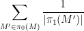
For a finite multiply-connected groupoid, it turns out that the natural notion of “cardinality” (or as I prefer to call it, “cardinality up to isomorphism”) is given by the variant

of (1). That is to say, in the multiply connected case, the denominator is no longer the number of objects ![{[x]}](https://s0.wp.com/latex.php?latex=%7B%5Bx%5D%7D&bg=ffffff&fg=000000&s=0&c=20201002)
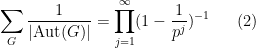
![\displaystyle \sum_{[x] \in X/\sim} \frac{1}{|\mathrm{Aut}(x)|} \ \ \ \ \ (2)](https://s0.wp.com/latex.php?latex=%5Cdisplaystyle+%5Csum_%7B%5Bx%5D+%5Cin+X%2F%5Csim%7D+%5Cfrac%7B1%7D%7B%7C%5Cmathrm%7BAut%7D%28x%29%7C%7D+%5C+%5C+%5C+%5C+%5C+%282%29&bg=ffffff&fg=000000&s=0&c=20201002)
where 


For instance, if we take
exactly as before. If however we take the multiply connected groupoid on

the equivalence class ![{[0]}](https://s0.wp.com/latex.php?latex=%7B%5B0%5D%7D&bg=ffffff&fg=000000&s=0&c=20201002)
![{[1], [2]}](https://s0.wp.com/latex.php?latex=%7B%5B1%5D%2C+%5B2%5D%7D&bg=ffffff&fg=000000&s=0&c=20201002)


The definition (2) can also make sense for some infinite groupoids; to my knowledge this was first explicitly done in this paper of Baez and Dolan. Consider for instance the category 


(This fact is sometimes loosely stated as “the number of finite sets is 

because the cyclic group
In the case that the cardinality of a groupoid
![\displaystyle {\mathbf P}([\mathbf{x}] = [x]) = \frac{1 / |\mathrm{Aut}(x)|}{\sum_{[y] \in X/\sim} 1/|\mathrm{Aut}(y)|},](https://s0.wp.com/latex.php?latex=%5Cdisplaystyle+%7B%5Cmathbf+P%7D%28%5B%5Cmathbf%7Bx%7D%5D+%3D+%5Bx%5D%29+%3D+%5Cfrac%7B1+%2F+%7C%5Cmathrm%7BAut%7D%28x%29%7C%7D%7B%5Csum_%7B%5By%5D+%5Cin+X%2F%5Csim%7D+1%2F%7C%5Cmathrm%7BAut%7D%28y%29%7C%7D%2C&bg=ffffff&fg=000000&s=0&c=20201002)
thus the probability of being isomorphic to a given element ![{[0], [1], [2]}](https://s0.wp.com/latex.php?latex=%7B%5B0%5D%2C+%5B1%5D%2C+%5B2%5D%7D&bg=ffffff&fg=000000&s=0&c=20201002)

![{[1]}](https://s0.wp.com/latex.php?latex=%7B%5B1%5D%7D&bg=ffffff&fg=000000&s=0&c=20201002)
![{[2]}](https://s0.wp.com/latex.php?latex=%7B%5B2%5D%7D&bg=ffffff&fg=000000&s=0&c=20201002)

Using the groupoid of finite sets, we see that a finite set chosen uniformly up to isomorphism will have a cardinality that is distributed according to the Poisson distribution of parameter 
One important source of groupoids are the fundamental groupoids 
where 


This notion of cardinality up to isomorphism of a groupoid behaves well with respect to various basic notions. For instance, suppose one has an 


![{[\mathrm{x}]}](https://s0.wp.com/latex.php?latex=%7B%5B%5Cmathrm%7Bx%7D%5D%7D&bg=ffffff&fg=000000&s=0&c=20201002)
![{\pi([\mathrm{x}])}](https://s0.wp.com/latex.php?latex=%7B%5Cpi%28%5B%5Cmathrm%7Bx%7D%5D%29%7D&bg=ffffff&fg=000000&s=0&c=20201002)
Indeed, one can show that this notion of cardinality up to isomorphism for groupoids is uniquely determined by a small number of axioms such as these (similar to the axioms that determine Euler characteristic); see this blog post of Qiaochu Yuan for details.
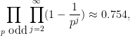
The probability distributions on isomorphism classes described by the above recipe seem to arise naturally in many applications. For instance, if one draws a profinite abelian group up to isomorphism at random in this fashion (so that each isomorphism class ![{[G]}](https://s0.wp.com/latex.php?latex=%7B%5BG%5D%7D&bg=ffffff&fg=000000&s=0&c=20201002)
I’ve just uploaded to the arXiv my paper “An integration approach to the Toeplitz square peg problem“, submitted to Forum of Mathematics, Sigma. This paper resulted from my attempts recently to solve the Toeplitz square peg problem (also known as the inscribed square problem):
Conjecture 1 (Toeplitz square peg problem) Let
See this recent survey of Matschke in the Notices of the AMS for the latest results on this problem.
The route I took to the results in this paper was somewhat convoluted. I was motivated to look at this problem after lecturing recently on the Jordan curve theorem in my class. The problem is superficially similar to the Jordan curve theorem in that the result is known (and rather easy to prove) if 


Inspired by my previous work on finite time blowup for various PDEs, I first tried looking for a counterexample in the category of (locally) self-similar curves that are smooth (or piecewise linear) away from a single origin where it can oscillate infinitely often; this is basically the smoothest type of curve that was not already covered by previous results. By a rescaling and compactness argument, it is not difficult to see that such a counterexample would exist if there was a counterexample to the following periodic version of the conjecture:
Conjecture 2 (Periodic square peg problem) Let
be two disjoint simple closed piecewise linear curves in the cylinder
which have a winding number of one, that is to say they are homologous to the loop
from
to
and
contains the four vertices of a square.
In contrast to Conjecture 1, which is known for polygonal paths, Conjecture 2 is still open even under the hypothesis of polygonal paths; the homological arguments alluded to previously now show that the number of inscribed squares in the periodic setting is even rather than odd, which is not enough to conclude the conjecture. (This flipping of parity from odd to even due to an infinite amount of oscillation is reminiscent of the “Eilenberg-Mazur swindle“, discussed in this previous post.)
I therefore tried to construct counterexamples to Conjecture 2. I began perturbatively, looking at curves 
![{\{ (t,f(t)): t \in [t_0,t_1]\} \cup \{ (t,g(t)): t \in [t_0,t_1]\}}](https://s0.wp.com/latex.php?latex=%7B%5C%7B+%28t%2Cf%28t%29%29%3A+t+%5Cin+%5Bt_0%2Ct_1%5D%5C%7D+%5Ccup+%5C%7B+%28t%2Cg%28t%29%29%3A+t+%5Cin+%5Bt_0%2Ct_1%5D%5C%7D%7D&bg=ffffff&fg=000000&s=0&c=20201002) of the graphs of two Lipschitz functions
of the graphs of two Lipschitz functions ![{f,g: [t_0,t_1] \rightarrow {\bf R}}](https://s0.wp.com/latex.php?latex=%7Bf%2Cg%3A+%5Bt_0%2Ct_1%5D+%5Crightarrow+%7B%5Cbf+R%7D%7D&bg=ffffff&fg=000000&s=0&c=20201002) of Lipschitz constant less than one that agree at the endpoints.
of Lipschitz constant less than one that agree at the endpoints.  of Lipschitz constant less than one.
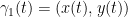
We sketch the proof of Theorem 3(i) as follows (the proof of Theorem 3(ii) is very similar). Let ![{\gamma_1: [t_0, t_1] \rightarrow {\bf R}}](https://s0.wp.com/latex.php?latex=%7B%5Cgamma_1%3A+%5Bt_0%2C+t_1%5D+%5Crightarrow+%7B%5Cbf+R%7D%7D&bg=ffffff&fg=000000&s=0&c=20201002)
![{t \in [t_0,t_1]}](https://s0.wp.com/latex.php?latex=%7Bt+%5Cin+%5Bt_0%2Ct_1%5D%7D&bg=ffffff&fg=000000&s=0&c=20201002)


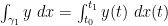
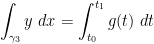
Now for the conserved integral of motion. If we integrate the 

This identity can be established by the following calculation: one can parameterise


for some Lipschitz functions ![{x,y,a,b: [t_0,t_1] \rightarrow {\bf R}}](https://s0.wp.com/latex.php?latex=%7Bx%2Cy%2Ca%2Cb%3A+%5Bt_0%2Ct_1%5D+%5Crightarrow+%7B%5Cbf+R%7D%7D&bg=ffffff&fg=000000&s=0&c=20201002)
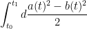
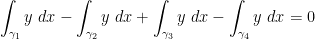
which vanishes because 

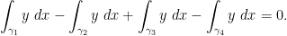
Using this conserved integral of motion, one can show that
which by Stokes’ theorem then implies that the bounded open region
This argument hinged on the curve 
Conjecture 4 (Area formulation of square peg problem) Let
be simple closed piecewise linear curves of winding number
(note the
are allowed to cross each other.) Then there exists a (possibly degenerate) square with vertices (traversed in anticlockwise order) lying on
It is not difficult to see that Conjecture 4 implies Conjecture 2. Actually I believe that the converse implication is at least morally true, in that any counterexample to Conjecture 4 can be eventually transformed to a counterexample to Conjecture 2 and Conjecture 1. The conserved integral of motion argument can establish Conjecture 4 in many cases, for instance if 
Conjecture 4 has a model special case, when one of the 
Conjecture 5 (Special case of area formulation) Let
be simple closed piecewise linear curves of winding number
Then there exist
and
with
such that
for
.

This conjecture is easy to establish if one of the curves, say 


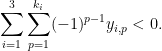
Using some elementary homological arguments (e.g. breaking up closed 

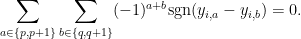
Conjecture 6 (Combinatorial form) Let
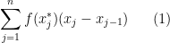
be odd natural numbers, and for each
be distinct real numbers; we adopt the convention that
. Assume the following axioms:
- (i) For any
, the sums
are non-zero.
- (ii) (Non-crossing) For any
with the same parity, the pairs
and
are non-crossing in the sense that
- (iii) (Non-crossing sums) For any
,
,
of the same parity, one has
Then one has

Roughly speaking, Conjecture 6 and Conjecture 5 are connected by constructing curves 


Using various ad hoc arguments involving “winding numbers”, it is possible to prove this conjecture in many cases (e.g. if one of the 

While I was not able to resolve the square peg problem, I think these results do provide a roadmap to attacking it, first by focusing on the combinatorial conjecture in Conjecture 6 (or its equivalent form in Conjecture 5), then after that is resolved moving on to Conjecture 4, and then finally to Conjecture 1.
Previous set of notes: Notes 1. Next set of notes: Notes 3.
Having discussed differentiation of complex mappings in the preceding notes, we now turn to the integration of complex maps. We first briefly review the situation of integration of (suitably regular) real functions ![{f: [a,b] \rightarrow {\bf R}}](https://s0.wp.com/latex.php?latex=%7Bf%3A+%5Ba%2Cb%5D+%5Crightarrow+%7B%5Cbf+R%7D%7D&bg=ffffff&fg=000000&s=0&c=20201002)
- (i) The signed definite integral
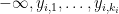
, which is usually interpreted as the Riemann integral (or equivalently, the Darboux integral), which can be defined as the limit (if it exists) of the Riemann sums
whereis some partition of
,
is an element of the interval
, and the limit is taken as the maximum mesh size
goes to zero (this can be formalised using the concept of a net). It is convenient to adopt the convention that
for
; alternatively one can interpret
as the limit of the Riemann sums (1), where now the (reversed) partition
goes leftwards from
- (ii) The unsigned definite integral
, usually interpreted as the Lebesgue integral. The precise definition of this integral is a little complicated (see e.g. this previous post), but roughly speaking the idea is to approximate
for some coefficients
and sets
, and then approximate the integral
, where
is the Lebesgue measure of
. In contrast to the signed definite integral, no orientation is imposed or used on the underlying domain of integration, which is viewed as an “undirected” set
- (iii) The indefinite integral or antiderivative
, defined as any function
whose derivative
exists and is equal to
, thus for instance
.
There are some other variants of the above integrals (e.g. the Henstock-Kurzweil integral, discussed for instance in this previous post), which can handle slightly different classes of functions and have slightly different properties than the standard integrals listed here, but we will not need to discuss such alternative integrals in this course (with the exception of some improper and principal value integrals, which we will encounter in later notes).
The above three notions of integration are closely related to each other. For instance, if
![\displaystyle \int_a^b f(x)\ dx = \int_{[a,b]} f(x)\ dx](https://s0.wp.com/latex.php?latex=%5Cdisplaystyle++%5Cint_a%5Eb+f%28x%29%5C+dx+%3D+%5Cint_%7B%5Ba%2Cb%5D%7D+f%28x%29%5C+dx&bg=ffffff&fg=000000&s=0&c=20201002)
and
![\displaystyle \int_b^a f(x)\ dx = -\int_{[a,b]} f(x)\ dx](https://s0.wp.com/latex.php?latex=%5Cdisplaystyle++%5Cint_b%5Ea+f%28x%29%5C+dx+%3D+-%5Cint_%7B%5Ba%2Cb%5D%7D+f%28x%29%5C+dx&bg=ffffff&fg=000000&s=0&c=20201002)
If 
for any ![{c,d \in [a,b]}](https://s0.wp.com/latex.php?latex=%7Bc%2Cd+%5Cin+%5Ba%2Cb%5D%7D&bg=ffffff&fg=000000&s=0&c=20201002)


All three of the above integration concepts have analogues in complex analysis. By far the most important notion will be the complex analogue of the signed definite integral, namely the contour integral 


As it turns out, the fundamental theorem of calculus continues to hold in the complex plane: under suitable regularity assumptions on a complex function
whenever 

Read the rest of this entry »
Bill Thurston, who made fundamental contributions to our understanding of low-dimensional manifolds and related structures, died on Tuesday, aged 65.
Perhaps Thurston’s best known achievement is the proof of the hyperbolisation theorem for Haken manifolds, which showed that 3-manifolds which obeyed a certain number of topological conditions, could always be given a hyperbolic geometry (i.e. a Riemannian metric that made the manifold isometric to a quotient of the hyperbolic 3-space 
One of my favourite results of Thurston’s is his elegant method for everting the sphere (smoothly turning a sphere 

In addition to his direct mathematical research contributions, Thurston was also an amazing mathematical expositor, having the rare knack of being able to describe the process of mathematical thinking in addition to the results of that process and the intuition underlying it. His wonderful essay “On proof and progress in mathematics“, which I highly recommend, is the quintessential instance of this; more recent examples include his many insightful questions and answers on MathOverflow.
I unfortunately never had the opportunity to meet Thurston in person (although we did correspond a few times online), but I know many mathematicians who have been profoundly influenced by him and his work. His death is a great loss for mathematics.
A topological space 

There are some obvious necessary conditions on the space 

In the converse direction, being Hausdorff and first countable is not always enough to guarantee metrisability, for a variety of reasons. For instance the long line is not metrisable despite being both Hausdorff and first countable, due to a failure of paracompactness, which prevents one from gluing together the local metric structures on this line into a global one. Even after adding in paracompactness, this is still not enough; the real line with the lower limit topology (also known as the Sorgenfrey line) is Hausdorff, first countable, and paracompact, but still not metrisable (because of a failure of second countability despite being separable).
However, there is one important setting in which the Hausdorff and first countability axioms do suffice to give metrisability, and that is the setting of topological groups:
Theorem 1 (Birkhoff-Kakutani theorem) Let
and
are continuous). Then
Remark 1 It is not hard to show that a topological group is Hausdorff if and only if the singleton set
is closed. More generally, in an arbitrary topological group, it is a good exercise to show that the closure of
is then a Hausdorff topological group. Because of this, the study of topological groups can usually be reduced immediately to the study of Hausdorff topological groups. (Indeed, in many texts, topological groups are automatically understood to be an abbreviation for “Hausdorff topological group”.)
The standard proof of the Birkhoff-Kakutani theorem (which we have taken from this book of Montgomery and Zippin) relies on the following Urysohn-type lemma:
Lemma 2 (Urysohn-type lemma) Let
with the following properties:
- (Unique maximum)
, and
for all
.
- (Neighbourhood base) The sets
for
- (Uniform continuity) For every
, there exists an open neighbourhood
of the identity such that
for all
and
.
Note that if 
Let us assume Lemma 2 for now and finish the proof of the Birkhoff-Kakutani theorem. We only prove the difficult direction, namely that a Hausdorff first countable topological group 

where 

Clearly 


To put it another way: because 

Now we have to check whether the metric 
To verify the former claim, it suffices to show that the map 
Remark 2 The above argument in fact shows that if a group
Now we prove Lemma 2. By first countability, we can find a countable neighbourhood base
of the identity. As

Using the continuity of the group axioms, we can recursively find a sequence of nested open neighbourhoods of the identity

such that each 


For every dyadic rational 


where 

for all 

We now set

with the understanding that 
Remark 3 A very similar argument to the one above also establishes that every topological group
Notice that the function 


- (Continuity)
and
are continuous on their domains of definition.
- (Identity) For any
,
and
are well-defined and equal to
- (Inverse) For any
,
and
are well-defined and equal to
is well-defined and equal to
- (Local associativity) If
are such that
,
,
, and
are all well-defined, then
.
Informally, one can view a local group as a topological group in which the closure axiom has been almost completely dropped, but with all the other axioms retained. A basic way to generate a local group is to start with an ordinary topological group 

Remark 4 Another important example of a local group is that of a group chunk, in which the sets
Zariski-open, and the group operations birational on their domains of definition. This is somewhat analogous to the notion of a “
group” in additive combinatorics. There are a number of group chunk theorems, starting with a theorem of Weil in the algebraic setting, which roughly speaking assert that a generic portion of a group chunk can be identified with the generic portion of a genuine group.
We then have
Theorem 3 (Birkhoff-Kakutani theorem for local groups) Let
of the identity which is metrisable.
Proof: (Sketch) It is not difficult to see that in a local group 


My motivation for studying local groups is that it turns out that there is a correspondence (first observed by Hrushovski) between the concept of an approximate group in additive combinatorics, and a locally compact local group in topological group theory; I hope to discuss this correspondence further in a subsequent post.
The ham sandwich theorem asserts that, given 


A useful generalisation of the ham sandwich theorem is the polynomial ham sandwich theorem, which asserts that given 


The polynomial ham sandwich theorem is a theorem about continuous bodies (bounded open sets), but a simple limiting argument leads one to the following discrete analogue: given 


Proposition 1 (Cell decomposition) Let
be a finite set of points in
of degree at most
into the hypersurface
of cells bounded by
, such that
, and such that each cell
contains at most
points.

A proof is sketched in this previous blog post. The cells in the argument are not necessarily connected (being instead formed by intersecting together a number of semi-algebraic sets such as 


Remark 1 By setting
, we obtain as a limiting case of the cell decomposition the fact that any finite set
The cell decomposition can be viewed as a structural theorem for arbitrary large configurations of points in space, much as the Szemerédi regularity lemma can be viewed as a structural theorem for arbitrary large dense graphs. Indeed, just as many problems in the theory of large dense graphs can be profitably attacked by first applying the regularity lemma and then inspecting the outcome, it now seems that many problems in combinatorial incidence geometry can be attacked by applying the cell decomposition (or a similar such decomposition), with a parameter
In this post, I wanted to record a simpler (but still illustrative) version of this method (that I learned from Nets Katz), namely to provide yet another proof of the Szemerédi-Trotter theorem in incidence geometry:
Theorem 2 (Szemerédi-Trotter theorem) Given a finite set of points
, the set of incidences
has cardinality

This theorem has many short existing proofs, including one via crossing number inequalities (as discussed in this previous post) or via a slightly different type of cell decomposition (as discussed here). The proof given below is not that different, in particular, from the latter proof, but I believe it still serves as a good introduction to the polynomial method in combinatorial incidence geometry.
Emmanuel Breuillard, Ben Green, and I have just uploaded to the arXiv our paper “Approximate subgroups of linear groups“, submitted to GAFA. This paper contains (the first part) of the results announced previously by us; the second part of these results, concerning expander groups, will appear subsequently. The release of this paper has been coordinated with the release of a parallel paper by Pyber and Szabo (previously announced within an hour(!) of our own announcement).
Our main result describes (with polynomial accuracy) the “sufficiently Zariski dense” approximate subgroups of simple algebraic groups 


Let 


Our first main theorem classifies the approximate subgroups
Theorem 1 (Approximate groups that generate) Let
or
, where the implied constants depend only on
The hypothesis that 
Theorem 2 (Zariski-dense approximate groups) Let
, where the implied constants depend only on
is the group generated by
Here, we say that an algebraic variety has complexity at most
In the case when 


Theorem 3 (Freiman’s theorem in
of size at most
, such that
translates of
This can be compared with Gromov’s celebrated theorem that any finitely generated group of polynomial growth is virtually nilpotent. Indeed, the above theorem easily implies Gromov’s theorem in the case of finitely generated subgroups of
By fairly standard arguments, the above classification theorems for approximate groups can be used to give bounds on the expansion and diameter of Cayley graphs, for instance one can establish a conjecture of Babai and Seress that connected Cayley graphs on absolutely almost simple groups over a finite field have polylogarithmic diameter at most. Applications to expanders include the result on Suzuki groups mentioned in a previous post; further applications will appear in a forthcoming paper.
Apart from the general structural theory of algebraic groups, and some quantitative analogues of the basic theory of algebraic geometry (which we chose to obtain via ultrafilters, as discussed in this post), we rely on two basic tools. Firstly, we use a version of the pivot argument developed first by Konyagin and Bourgain-Glibichuk-Konyagin in the setting of sum-product estimates, and generalised to more non-commutative settings by Helfgott; this is discussed in this previous post. Secondly, we adapt an argument of Larsen and Pink (which we learned from a paper of Hrushovski) to obtain a sharp bound on the extent to which a sufficiently Zariski-dense approximate groups can concentrate in a (bounded complexity) subvariety; this is discussed at the end of this blog post.
This week I was in my home town of Adelaide, Australia, for the 2009 annual meeting of the Australian Mathematical Society. This was a fairly large meeting (almost 500 participants). One of the highlights of such a large meeting is the ability to listen to plenary lectures in fields adjacent to one’s own, in which speakers can give high-level overviews of a subject without getting too bogged down in the technical details. From the talks here I learned a number of basic things which were well known to experts in that field, but which I had not fully appreciated, and so I wanted to share them here.
The first instance of this was from a plenary lecture by Danny Calegari entitled “faces of the stable commutator length (scl) ball”. One thing I learned from this talk is that in homotopy theory, there is a very close relationship between topological spaces (such as manifolds) on one hand, and groups (and generalisations of groups) on the other, so that homotopy-theoretic questions about the former can often be converted to purely algebraic questions about the latter, and vice versa; indeed, it seems that homotopy theorists almost think of topological spaces and groups as being essentially the same concept, despite looking very different at first glance. To get from a space 


This theme was reinforced by another plenary lecture by Ezra Getzler entitled “
Mohammed Abuzaid gave a plenary lecture entitled “Functoriality in homological mirror symmetry”. One thing I learned from this talk was that the (partially conjectural) phenomenon of (homological) mirror symmetry is one of several types of duality, in which the behaviour of maps into one mathematical object 

There was a related theme in a talk by Dennis Gaitsgory entitled “The geometric Langlands program”. From my (very superficial) understanding of the Langlands program, the behaviour of specific maps into a reductive Lie group 
Related also to this was a plenary talk by Akshay Venkatesh, entitled “The Cohen-Lenstra heuristics over global fields”. Here, the question concerned the conjectural behaviour of class groups of quadratic fields, and in particular to explain the numerically observed phenomenon that about 
![{{\Bbb Q}[\sqrt{d}]}](https://s0.wp.com/latex.php?latex=%7B%7B%5CBbb+Q%7D%5B%5Csqrt%7Bd%7D%5D%7D&bg=ffffff&fg=000000&s=0&c=20201002)


where 
where
Based on the heuristic that the class group should behave “randomly” subject to some “obvious” constraints, it is expected that a randomly chosen real quadratic field
whereas a randomly chosen imaginary quadratic field ![{{\Bbb Q}[\sqrt{-d}]}](https://s0.wp.com/latex.php?latex=%7B%7B%5CBbb+Q%7D%5B%5Csqrt%7B-d%7D%5D%7D&bg=ffffff&fg=000000&s=0&c=20201002)
The former claim is conjectural, whereas the latter claim follows from (for instance) Siegel’s theorem on the size of the class group, as discussed in this previous post. Ellenberg, Venkatesh, and Westerland have recently established some partial results towards the function field analogues of these heuristics.
One of the most important topological concepts in analysis is that of compactness (as discussed for instance in my Companion article on this topic). There are various flavours of this concept, but let us focus on sequential compactness: a subset E of a topological space X is sequentially compact if every sequence in E has a convergent subsequence whose limit is also in E. This property allows one to do many things with the set E. For instance, it allows one to maximise a functional on E:
Proposition 1. (Existence of extremisers) Let E be a non-empty sequentially compact subset of a topological space X, and let
be a continuous function. Then the supremum
is attained at at least one point
, thus
for all
. (In particular, this supremum is finite.) Similarly for the infimum.
Proof. Let 


Remark 1. An inspection of the argument shows that one can relax the continuity hypothesis on F somewhat: to attain the supremum, it suffices that F be upper semicontinuous, and to attain the infimum, it suffices that F be lower semicontinuous.

We thus see that sequential compactness is useful, among other things, for ensuring the existence of extremisers. In finite-dimensional spaces (such as vector spaces), compact sets are plentiful; indeed, the Heine-Borel theorem asserts that every closed and bounded set is compact. However, once one moves to infinite-dimensional spaces, such as function spaces, then the Heine-Borel theorem fails quite dramatically; most of the closed and bounded sets one encounters in a topological vector space are non-compact, if one insists on using a reasonably “strong” topology. This causes a difficulty in (among other things) calculus of variations, which is often concerned to finding extremisers to a functional
In recent decades, mathematicians have found a number of ways to get around this difficulty. One of them is to weaken the topology to recover compactness, taking advantage of such results as the Banach-Alaoglu theorem (or its sequential counterpart). Of course, there is a tradeoff: weakening the topology makes compactness easier to attain, but makes the continuity of F harder to establish. Nevertheless, if F enjoys enough “smoothing” or “cancellation” properties, one can hope to obtain continuity in the weak topology, allowing one to do things such as locate extremisers. (The phenomenon that cancellation can lead to continuity in the weak topology is sometimes referred to as compensated compactness.)
Another option is to abandon trying to make all sequences have convergent subsequences, and settle just for extremising sequences to have convergent subsequences, as this would still be enough to retain Theorem 1. Pursuing this line of thought leads to the Palais-Smale condition, which is a substitute for compactness in some calculus of variations situations.
But in many situations, one cannot weaken the topology to the point where the domain E becomes compact, without destroying the continuity (or semi-continuity) of F, though one can often at least find an intermediate topology (or metric) in which F is continuous, but for which E is still not quite compact. Thus one can find sequences
Nevertheless, even though a sequence 


In typical applications, the concentration compactness phenomenon is exploited in moderately sophisticated function spaces (such as Sobolev spaces or Strichartz spaces), with the failure of traditional compactness being connected to a moderately complicated group G of symmetries (e.g. the group generated by translations and dilations). Because of this, concentration compactness can appear to be a rather complicated and technical concept when it is first encountered. In this note, I would like to illustrate concentration compactness in a simple toy setting, namely in the space 


Recent Comments