You are currently browsing the category archive for the ‘275A – probability theory’ category.

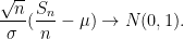
In the previous set of notes we established the central limit theorem, which we formulate here as follows:

Theorem 1 (Central limit theorem) Let {X_1,X_2,X_3,\dots} be iid copies of a real random variable {X} of mean {\mu} and variance {0 < \sigma^2 < \infty}, and write {S_n := X_1 + \dots + X_n}. Then, for any fixed {a < b}, we have

\displaystyle {\bf P}( a \leq \frac{S_n - n \mu}{\sqrt{n} \sigma} \leq b ) \rightarrow \frac{1}{\sqrt{2\pi}} \int_a^b e^{-t^2/2}\ dt \ \ \ \ \ (1)

as {n \rightarrow \infty}.

This is however not the end of the matter; there are many variants, refinements, and generalisations of the central limit theorem, and the purpose of this set of notes is to present a small sample of these variants.

First of all, the above theorem does not quantify the rate of convergence in (1). We have already addressed this issue to some extent with the Berry-Esséen theorem, which roughly speaking gives a convergence rate of {O(1/\sqrt{n})} uniformly in {a,b} if we assume that {X} has finite third moment. However there are still some quantitative versions of (1) which are not addressed by the Berry-Esséen theorem. For instance one may be interested in bounding the large deviation probabilities

\displaystyle {\bf P}( |\frac{S_n - n \mu}{\sqrt{n} \sigma}| \geq \lambda ) \ \ \ \ \ (2)

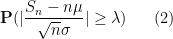
in the setting where {\lambda} grows with {n}. Chebyshev’s inequality gives an upper bound of {1/\lambda^2} for this quantity, but one can often do much better than this in practice. For instance, the central limit theorem (1) suggests that this probability should be bounded by something like {O( e^{-\lambda^2/2})}; however, this theorem only kicks in when {n} is very large compared with {\lambda}. For instance, if one uses the Berry-Esséen theorem, one would need {n} as large as {e^{\lambda^2}} or so to reach the desired bound of {O( e^{-\lambda^2/2})}, even under the assumption of finite third moment. Basically, the issue is that convergence-in-distribution results, such as the central limit theorem, only really control the typical behaviour of statistics in {\frac{S_n-n \mu}{\sqrt{n} \sigma}}; they are much less effective at controlling the very rare outlier events in which the statistic strays far from its typical behaviour. Fortunately, there are large deviation inequalities (or concentration of measure inequalities) that do provide exponential type bounds for quantities such as (2), which are valid for both small and large values of {n}. A basic example of this is the Chernoff bound that made an appearance in Exercise 47 of Notes 4; here we give some further basic inequalities of this type, including versions of the Bennett and Hoeffding inequalities.

In the other direction, we can also look at the fine scale behaviour of the sums {S_n} by trying to control probabilities such as

\displaystyle {\bf P}( a \leq S_n \leq a+h ) \ \ \ \ \ (3)

where {h} is now bounded (but {a} can grow with {n}). The central limit theorem predicts that this quantity should be roughly {\frac{h}{\sqrt{2\pi n} \sigma} e^{-(a-n\mu)^2 / 2n \sigma^2}}, but even if one is able to invoke the Berry-Esséen theorem, one cannot quite see this main term because it is dominated by the error term {O(1/n^{1/2})} in Berry-Esséen. There is good reason for this: if for instance {X} takes integer values, then {S_n} also takes integer values, and {{\bf P}( a \leq S_n \leq a+h )} can vanish when {h} is less than {1} and {a} is slightly larger than an integer. However, this turns out to essentially be the only obstruction; if {X} does not lie in a lattice such as {{\bf Z}}, then we can establish a local limit theorem controlling (3), and when {X} does take values in a lattice like {{\bf Z}}, there is a discrete local limit theorem that controls probabilities such as {{\bf P}(S_n = m)}. Both of these limit theorems will be proven by the Fourier-analytic method used in the previous set of notes.

We also discuss other limit theorems in which the limiting distribution is something other than the normal distribution. Perhaps the most common example of these theorems is the Poisson limit theorems, in which one sums a large number of indicator variables (or approximate indicator variables), each of which is rarely non-zero, but which collectively add up to a random variable of medium-sized mean. In this case, it turns out that the limiting distribution should be a Poisson random variable; this again is an easy application of the Fourier method. Finally, we briefly discuss limit theorems for other stable laws than the normal distribution, which are suitable for summing random variables of infinite variance, such as the Cauchy distribution.

Finally, we mention a very important class of generalisations to the CLT (and to the variants of the CLT discussed in this post), in which the hypothesis of joint independence between the variables {X_1,\dots,X_n} is relaxed, for instance one could assume only that the {X_1,\dots,X_n} form a martingale. Many (though not all) of the proofs of the CLT extend to these more general settings, and this turns out to be important for many applications in which one does not expect joint independence. However, we will not discuss these generalisations in this course, as they are better suited for subsequent courses in this series when the theory of martingales, conditional expectation, and related tools are developed.

Read the rest of this entry »

Let {X_1,X_2,\dots} be iid copies of an absolutely integrable real scalar random variable {X}, and form the partial sums {S_n := X_1 + \dots + X_n}. As we saw in the last set of notes, the law of large numbers ensures that the empirical averages {S_n/n} converge (both in probability and almost surely) to a deterministic limit, namely the mean {\mu= {\bf E} X} of the reference variable {X}. Furthermore, under some additional moment hypotheses on the underlying variable {X}, we can obtain square root cancellation for the fluctuation {\frac{S_n}{n} - \mu} of the empirical average from the mean. To simplify the calculations, let us first restrict to the case {\mu=0, \sigma^2=1} of mean zero and variance one, thus

\displaystyle  {\bf E} X = 0

and

\displaystyle  {\bf Var}(X) = {\bf E} X^2 = 1.

Then, as computed in previous notes, the normalised fluctuation {S_n/\sqrt{n}} also has mean zero and variance one:

\displaystyle  {\bf E} \frac{S_n}{\sqrt{n}} = 0

\displaystyle  {\bf Var}(\frac{S_n}{\sqrt{n}}) = {\bf E} (\frac{S_n}{\sqrt{n}})^2 = 1.

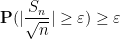
This and Chebyshev’s inequality already indicates that the “typical” size of {S_n} is {O(\sqrt{n})}, thus for instance {\frac{S_n}{\sqrt{n} \omega(n)}} goes to zero in probability for any {\omega(n)} that goes to infinity as {n \rightarrow \infty}. If we also have a finite fourth moment {{\bf E} |X|^4 < \infty}, then the calculations of the previous notes also give a fourth moment estimate

\displaystyle  {\bf E} (\frac{S_n}{\sqrt{n}})^4 = 3 + O( \frac{{\bf E} |X|^4}{n} ).

From this and the Paley-Zygmund inequality (Exercise 44 of Notes 1) we also get some lower bound for {\frac{S_n}{\sqrt{n}}} of the form

\displaystyle  {\bf P}( |\frac{S_n}{\sqrt{n}}| \geq \varepsilon ) \geq \varepsilon

for some absolute constant {\varepsilon>0} and for {n} sufficiently large; this indicates in particular that {\frac{S_n \omega(n)}{\sqrt{n}}} does not converge in any reasonable sense to something finite for any {\omega(n)} that goes to infinity.
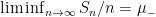
The question remains as to what happens to the ratio {S_n/\sqrt{n}} itself, without multiplying or dividing by any factor {\omega(n)}. A first guess would be that these ratios converge in probability or almost surely, but this is unfortunately not the case:

Proposition 1 Let {X_1,X_2,\dots} be iid copies of an absolutely integrable real scalar random variable {X} with mean zero, variance one, and finite fourth moment, and write {S_n := X_1 + \dots + X_n}. Then the random variables {S_n/\sqrt{n}} do not converge in probability or almost surely to any limit, and neither does any subsequence of these random variables.

Proof: Suppose for contradiction that some sequence {S_{n_j}/\sqrt{n_j}} converged in probability or almost surely to a limit {Y}. By passing to a further subsequence we may assume that the convergence is in the almost sure sense. Since all of the {S_{n_j}/\sqrt{n_j}} have mean zero, variance one, and bounded fourth moment, Theorem 25 of Notes 1 implies that the limit {Y} also has mean zero and variance one. On the other hand, {Y} is a tail random variable and is thus almost surely constant by the Kolmogorov zero-one law from Notes 3. Since constants have variance zero, we obtain the required contradiction. \Box

Nevertheless there is an important limit for the ratio {S_n/\sqrt{n}}, which requires one to replace the notions of convergence in probability or almost sure convergence by the weaker concept of convergence in distribution.

Definition 2 (Vague convergence and convergence in distribution) Let {R} be a locally compact Hausdorff topological space with the Borel {\sigma}-algebra. A sequence of finite measures {\mu_n} on {R} is said to converge vaguely to another finite measure {\mu} if one has

\displaystyle  \int_R G(x)\ d\mu_n(x) \rightarrow \int_R G(x)\ d\mu(x)

as {n \rightarrow \infty} for all continuous compactly supported functions {G: R \rightarrow {\bf R}}. (Vague convergence is also known as weak convergence, although strictly speaking the terminology weak-* convergence would be more accurate.) A sequence of random variables {X_n} taking values in {R} is said to converge in distribution (or converge weakly or converge in law) to another random variable {X} if the distributions {\mu_{X_n}} converge vaguely to the distribution {\mu_X}, or equivalently if

\displaystyle  {\bf E}G(X_n) \rightarrow {\bf E} G(X)

as {n \rightarrow \infty} for all continuous compactly supported functions {G: R \rightarrow {\bf R}}.

One could in principle try to extend this definition beyond the locally compact Hausdorff setting, but certain pathologies can occur when doing so (e.g. failure of the Riesz representation theorem), and we will never need to consider vague convergence in spaces that are not locally compact Hausdorff, so we restrict to this setting for simplicity.

Note that the notion of convergence in distribution depends only on the distribution of the random variables involved. One consequence of this is that convergence in distribution does not produce unique limits: if {X_n} converges in distribution to {X}, and {Y} has the same distribution as {X}, then {X_n} also converges in distribution to {Y}. However, limits are unique up to equivalence in distribution (this is a consequence of the Riesz representation theorem, discussed for instance in this blog post). As a consequence of the insensitivity of convergence in distribution to equivalence in distribution, we may also legitimately talk about convergence of distribution of a sequence of random variables {X_n} to another random variable {X} even when all the random variables {X_1,X_2,\dots} and {X} involved are being modeled by different probability spaces (e.g. each {X_n} is modeled by {\Omega_n}, and {X} is modeled by {\Omega}, with no coupling presumed between these spaces). This is in contrast to the stronger notions of convergence in probability or almost sure convergence, which require all the random variables to be modeled by a common probability space. Also, by an abuse of notation, we can say that a sequence {X_n} of random variables converges in distribution to a probability measure {\mu}, when {\mu_{X_n}} converges vaguely to {\mu}. Thus we can talk about a sequence of random variables converging in distribution to a uniform distribution, a gaussian distribution, etc..

From the dominated convergence theorem (available for both convergence in probability and almost sure convergence) we see that convergence in probability or almost sure convergence implies convergence in distribution. The converse is not true, due to the insensitivity of convergence in distribution to equivalence in distribution; for instance, if {X_1,X_2,\dots} are iid copies of a non-deterministic scalar random variable {X}, then the {X_n} trivially converge in distribution to {X}, but will not converge in probability or almost surely (as one can see from the zero-one law). However, there are some partial converses that relate convergence in distribution to convergence in probability; see Exercise 10 below.

Remark 3 The notion of convergence in distribution is somewhat similar to the notion of convergence in the sense of distributions that arises in distribution theory (discussed for instance in this previous blog post), however strictly speaking the two notions of convergence are distinct and should not be confused with each other, despite the very similar names.

The notion of convergence in distribution simplifies in the case of real scalar random variables:

Proposition 4 Let {X_1,X_2,\dots} be a sequence of scalar random variables, and let {X} be another scalar random variable. Then the following are equivalent:

  • (i) {X_n} converges in distribution to {X}.
  • (ii) {F_{X_n}(t)} converges to {F_X(t)} for each continuity point {t} of {F_X} (i.e. for all real numbers {t \in {\bf R}} at which {F_X} is continuous). Here {F_X(t) := {\bf P}(X \leq t)} is the cumulative distribution function of {X}.

Proof: First suppose that {X_n} converges in distribution to {X}, and {F_X} is continuous at {t}. For any {\varepsilon > 0}, one can find a {\delta} such that

\displaystyle  F_X(t) - \varepsilon \leq F_X(t') \leq F_X(t) + \varepsilon

for every {t' \in [t-\delta,t+\delta]}. One can also find an {N} larger than {|t|+\delta} such that {F_X(-N) \leq \varepsilon} and {F_X(N) \geq 1-\varepsilon}. Thus

\displaystyle  {\bf P} (|X| \geq N ) = O(\varepsilon)

and

\displaystyle  {\bf P} (|X - t| \leq \delta ) = O(\varepsilon).

Let {G: {\bf R} \rightarrow [0,1]} be a continuous function supported on {[-2N, t]} that equals {1} on {[-N, t-\delta]}. Then by the above discussion we have

\displaystyle  {\bf E} G(X) = F_X(t) + O(\varepsilon)

and hence

\displaystyle  {\bf E} G(X_n) = F_X(t) + O(\varepsilon)

for large enough {n}. In particular

\displaystyle  {\bf P}( X_n \leq t ) \geq F_X(t) - O(\varepsilon).

A similar argument, replacing {G} with a continuous function supported on {[t,2N]} that equals {1} on {[t+\delta,N]} gives

\displaystyle  {\bf P}( X_n > t ) \geq 1 - F_X(t) - O(\varepsilon)

for {n} large enough. Putting the two estimates together gives

\displaystyle  F_{X_n}(t) = F_X(t) + O(\varepsilon)

for {n} large enough; sending {\varepsilon \rightarrow 0}, we obtain the claim.
Conversely, suppose that {F_{X_n}(t)} converges to {F_X(t)} at every continuity point {t} of {F_X}. Let {G: {\bf R} \rightarrow {\bf R}} be a continuous compactly supported function, then it is uniformly continuous. As {F_X} is monotone increasing, it can only have countably many points of discontinuity. From these two facts one can find, for any {\varepsilon>0}, a simple function {G_\varepsilon(t) = \sum_{i=1}^n c_i 1_{(t_i,t_{i+1}]}} for some {t_1 < \dots < t_n} that are points of continuity of {F_X}, and real numbers {c_i}, such that {|G(t) - G_\varepsilon(t)| \leq \varepsilon} for all {t}. Thus

\displaystyle  {\bf E} G(X_n) = {\bf E} G_\varepsilon(X_n) + O(\varepsilon)

\displaystyle  = \sum_{i=1}^n c_i(F_{X_n}(t_{i+1}) - F_{X_n}(t)) + O(\varepsilon).

Similarly for {X_n} replaced by {X}. Subtracting and taking limit superior, we conclude that

\displaystyle  \limsup_{n \rightarrow \infty} |{\bf E} G(X_n) - {\bf E} G(X)| = O(\varepsilon),

and on sending {\varepsilon \rightarrow 0}, we obtain that {X_n} converges in distribution to {X} as claimed. \Box
The restriction to continuity points of {t} is necessary. Consider for instance the deterministic random variables {X_n = 1/n}, then {X_n} converges almost surely (and hence in distribution) to {0}, but {F_{X_n}(0) = 0} does not converge to {F_X(0)=1}.

Example 5 For any natural number {n}, let {X_n} be a discrete random variable drawn uniformly from the finite set {\{0/n, 1/n, \dots, (n-1)/n\}}, and let {X} be the continuous random variable drawn uniformly from {[0,1]}. Then {X_n} converges in distribution to {X}. Thus we see that a continuous random variable can emerge as the limit of discrete random variables.

Example 6 For any natural number {n}, let {X_n} be a continuous random variable drawn uniformly from {[0,1/n]}, then {X_n} converges in distribution to the deterministic real number {0}. Thus we see that discrete (or even deterministic) random variables can emerge as the limit of continuous random variables.

Exercise 7 (Portmanteau theorem) Show that the properties (i) and (ii) in Proposition 4 are also equivalent to the following three statements:

  • (iii) One has {\limsup_{n \rightarrow \infty} {\bf P}( X_n \in K ) \leq {\bf P}(X \in K)} for all closed sets {K \subset {\bf R}}.
  • (iv) One has {\liminf_{n \rightarrow \infty} {\bf P}( X_n \in U ) \geq {\bf P}(X \in U)} for all open sets {U \subset {\bf R}}.
  • (v) For any Borel set {E \subset {\bf R}} whose topological boundary {\partial E} is such that {{\bf P}(X \in \partial E) = 0}, one has {\lim_{n \rightarrow \infty} {\bf P}(X_n \in E) = {\bf P}(X \in E)}.

(Note: to prove this theorem, you may wish to invoke Urysohn’s lemma. To deduce (iii) from (i), you may wish to start with the case of compact {K}.)

We can now state the famous central limit theorem:

Theorem 8 (Central limit theorem) Let {X_1,X_2,\dots} be iid copies of a scalar random variable {X} of finite mean {\mu := {\bf E} X} and finite non-zero variance {\sigma^2 := {\bf Var}(X)}. Let {S_n := X_1 + \dots + X_n}. Then the random variables {\frac{\sqrt{n}}{\sigma} (\frac{S_n}{n} - \mu)} 
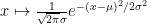
converges in distribution to a random variable with the standard normal distribution {N(0,1)} (that is to say, a random variable with probability density function {x \mapsto \frac{1}{\sqrt{2\pi}} e^{-x^2/2}}). Thus, by abuse of notation

\displaystyle  \frac{\sqrt{n}}{\sigma} (\frac{S_n}{n} - \mu) \rightarrow N(0,1).

In the normalised case {\mu=0, \sigma^2=1} when {X} has mean zero and unit variance, this simplifies to

\displaystyle  \frac{S_n}{\sqrt{n}} \rightarrow N(0,1).

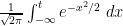
Using Proposition 4 (and the fact that the cumulative distribution function associated to {N(0,1)} is continuous, the central limit theorem is equivalent to asserting that

\displaystyle  {\bf P}( \frac{\sqrt{n}}{\sigma} (\frac{S_n}{n} - \mu) \leq t ) \rightarrow \frac{1}{\sqrt{2\pi}} \int_{-\infty}^t e^{-x^2/2}\ dx

as {n \rightarrow \infty} for any {t \in {\bf R}}, or equivalently that

\displaystyle  {\bf P}( a \leq \frac{\sqrt{n}}{\sigma} (\frac{S_n}{n} - \mu) \leq b ) \rightarrow \frac{1}{\sqrt{2\pi}} \int_{a}^b e^{-x^2/2}\ dx.

Informally, one can think of the central limit theorem as asserting that {S_n} approximately behaves like it has distribution {N( n \mu, n \sigma^2 )} for large {n}, where {N(\mu,\sigma^2)} is the normal distribution with mean {\mu} and variance {\sigma^2}, that is to say the distribution with probability density function {x \mapsto \frac{1}{\sqrt{2\pi} \sigma} e^{-(x-\mu)^2/2\sigma^2}}. The integrals {\frac{1}{\sqrt{2\pi}} \int_{-\infty}^t e^{-x^2/2}\ dx} can be written in terms of the error function {\hbox{erf}} as {\frac{1}{2} + \frac{1}{2} \hbox{erf}(t/\sqrt{2})}.
The central limit theorem is a basic example of the universality phenomenon in probability – many statistics involving a large system of many independent (or weakly dependent) variables (such as the normalised sums {\frac{\sqrt{n}}{\sigma}(\frac{S_n}{n}-\mu)}) end up having a universal asymptotic limit (in this case, the normal distribution), regardless of the precise makeup of the underlying random variable {X} that comprised that system. Indeed, the universality of the normal distribution is such that it arises in many other contexts than the fluctuation of iid random variables; the central limit theorem is merely the first place in probability theory where it makes a prominent appearance.

We will give several proofs of the central limit theorem in these notes; each of these proofs has their advantages and disadvantages, and can each extend to prove many further results beyond the central limit theorem. We first give Lindeberg’s proof of the central limit theorem, based on exchanging (or swapping) each component {X_1,\dots,X_n} of the sum {S_n} in turn. This proof gives an accessible explanation as to why there should be a universal limit for the central limit theorem; one then computes directly with gaussians to verify that it is the normal distribution which is the universal limit. Our second proof is the most popular one taught in probability texts, namely the Fourier-analytic proof based around the concept of the characteristic function {t \mapsto {\bf E} e^{itX}} of a real random variable {X}. Thanks to the powerful identities and other results of Fourier analysis, this gives a quite short and direct proof of the central limit theorem, although the arguments may seem rather magical to readers who are not already familiar with Fourier methods. Finally, we give a proof based on the moment method, in the spirit of the arguments in the previous notes; this argument is more combinatorial, but is straightforward and is particularly robust, in particular being well equipped to handle some dependencies between components; we will illustrate this by proving the Erdos-Kac law in number theory by this method. Some further discussion of the central limit theorem (including some further proofs, such as one based on Stein’s method) can be found in this blog post. Some further variants of the central limit theorem, such as local limit theorems, stable laws, and large deviation inequalities, will be discussed in the next (and final) set of notes.

The following exercise illustrates the power of the central limit theorem, by establishing combinatorial estimates which would otherwise require the use of Stirling’s formula to establish.

Exercise 9 (De Moivre-Laplace theorem) Let {X} be a Bernoulli random variable, taking values in {\{0,1\}} with {{\bf P}(X=0)={\bf P}(X=1)=1/2}, thus {X} has mean {1/2} and variance {1/4}. Let {X_1,X_2,\dots} be iid copies of {X}, and write {S_n := X_1+\dots+X_n}.

  • (i) Show that {S_n} takes values in {\{0,\dots,n\}} with {{\bf P}(S_n=i) = \frac{1}{2^n} \binom{n}{i}}. (This is an example of a binomial distribution.)
  • (ii) Assume Stirling’s formula

    \displaystyle  n! = (1+o(1)) \sqrt{2\pi n} n^n e^{-n} \ \ \ \ \ (1)

    where {o(1)} is a function of {n} that goes to zero as {n \rightarrow \infty}. (A proof of this formula may be found in this previous blog post.) Using this formula, and without using the central limit theorem, show that

    \displaystyle  {\bf P}( a \leq 2\sqrt{n} (\frac{S_n}{n} - \frac{1}{2}) \leq b ) \rightarrow \frac{1}{\sqrt{2\pi}} \int_{a}^b e^{-x^2/2}\ dx

    as {n \rightarrow \infty} for any fixed real numbers {a<b}.

The above special case of the central limit theorem was first established by de Moivre and Laplace.

We close this section with some basic facts about convergence of distribution that will be useful in the sequel.

Exercise 10 Let {X_1,X_2,\dots}, {Y_1,Y_2,\dots} be sequences of real random variables, and let {X,Y} be further real random variables.

  • (i) If {X} is deterministic, show that {X_n} converges in distribution to {X} if and only if {X_n} converges in probability to {X}.
  • (ii) Suppose that {X_n} is independent of {Y_n} for each {n}, and {X} independent of {Y}. Show that {X_n+iY_n} converges in distribution to {X+iY} if and only if {X_n} converges in distribution to {X} and {Y_n} converges in distribution to {Y}. (The shortest way to prove this is by invoking the Stone-Weierstrass theorem, but one can also proceed by proving some version of Proposition 4.) What happens if the independence hypothesis is dropped?
  • (iii) If {X_n} converges in distribution to {X}, show that for every {\varepsilon>0} there exists {K>0} such that {{\bf P}( |X_n| \geq K ) < \varepsilon} for all sufficiently large {n}. (That is to say, {X_n} is a tight sequence of random variables.)
  • (iv) Show that {X_n} converges in distribution to {X} if and only if, after extending the probability space model if necessary, one can find copies {Z_1,Z_2,\dots} and {Z} of {X_1,X_2,\dots} and {X} respectively such that {Z_n} converges almost surely to {Z}. (Hint: use the Skorohod representation, Exercise 29 of Notes 0.)
  • (v) If {X_1,X_2,\dots} converges in distribution to {X}, and {F: {\bf R} \rightarrow {\bf R}} is continuous, show that {F(X_1),F(X_2),\dots} converges in distribution to {F(X)}. Generalise this claim to the case when {X} takes values in an arbitrary locally compact Hausdorff space.
  • (vi) (Slutsky’s theorem) If {X_n} converges in distribution to {X}, and {Y_n} converges in probability to a deterministic limit {Y}, show that {X_n+Y_n} converges in distribution to {X+Y}, and {X_n Y_n} converges in distribution to {XY}. (Hint: either use (iv), or else use (iii) to control some error terms.) This statement combines particularly well with (i). What happens if {Y} is not assumed to be deterministic?
  • (vii) (Fatou lemma) If {G: {\bf R} \rightarrow [0,+\infty)} is continuous, and {X_n} converges in distribution to {X}, show that {\liminf_{n \rightarrow \infty} {\bf E} G(X_n) \geq {\bf E} G(X)}.
  • (viii) (Bounded convergence) If {G: {\bf R} \rightarrow {\bf R}} is continuous and bounded, and {X_n} converges in distribution to {X}, show that {\lim_{n \rightarrow \infty} {\bf E} G(X_n) = {\bf E} G(X)}.
  • (ix) (Dominated convergence) If {X_n} converges in distribution to {X}, and there is an absolutely integrable {Y} such that {|X_n| \leq Y} almost surely for all {n}, show that {\lim_{n \rightarrow \infty} {\bf E} X_n = {\bf E} X}.

For future reference we also mention (but will not prove) Prokhorov’s theorem that gives a partial converse to part (iii) of the above exercise:

Theorem 11 (Prokhorov’s theorem) Let {X_1,X_2,\dots} be a sequence of real random variables which is tight (that is, for every {\varepsilon>0} there exists {K>0} such that {{\bf P}(|X_n| \geq K) < \varepsilon} for all sufficiently large {n}). Then there exists a subsequence {X_{n_j}} which converges in distribution to some random variable {X} (which may possibly be modeled by a different probability space model than the {X_1,X_2,\dots}.)

The proof of this theorem relies on the Riesz representation theorem, and is beyond the scope of this course; but see for instance Exercise 29 of this previous blog post. (See also the closely related Helly selection theorem, covered in Exercise 30 of the same post.)

Read the rest of this entry »

One of the major activities in probability theory is studying the various statistics that can be produced from a complex system with many components. One of the simplest possible systems one can consider is a finite sequence {X_1,\dots,X_n} or an infinite sequence {X_1,X_2,\dots} of jointly independent scalar random variables, with the case when the {X_i} are also identically distributed (i.e. the {X_i} are iid) being a model case of particular interest. (In some cases one may consider a triangular array {(X_{n,i})_{1 \leq i \leq n}} of scalar random variables, rather than a finite or infinite sequence.) There are many statistics of such sequences that one can study, but one of the most basic such statistics are the partial sums

\displaystyle  S_n := X_1 + \dots + X_n.

The first fundamental result about these sums is the law of large numbers (or LLN for short), which comes in two formulations, weak (WLLN) and strong (SLLN). To state these laws, we first must define the notion of convergence in probability.

Definition 1 Let {X_n} be a sequence of random variables taking values in a separable metric space {R = (R,d)} (e.g. the {X_n} could be scalar random variables, taking values in {{\bf R}} or {{\bf C}}), and let {X} be another random variable taking values in {R}. We say that {X_n} converges in probability to {X} if, for every radius {\varepsilon > 0}, one has {{\bf P}( d(X_n,X) > \varepsilon ) \rightarrow 0} as {n \rightarrow \infty}. Thus, if {X_n, X} are scalar, we have {X_n} converging to {X} in probability if {{\bf P}( |X_n-X| > \varepsilon ) \rightarrow 0} as {n \rightarrow \infty} for any given {\varepsilon > 0}.

The measure-theoretic analogue of convergence in probability is convergence in measure.
It is instructive to compare the notion of convergence in probability with almost sure convergence. it is easy to see that {X_n} converges almost surely to {X} if and only if, for every radius {\varepsilon > 0}, one has {{\bf P}( \bigvee_{n \geq N} (d(X_n,X)>\varepsilon) ) \rightarrow 0} as {N \rightarrow \infty}; thus, roughly speaking, convergence in probability is good for controlling how a single random variable {X_n} is close to its putative limiting value {X}, while almost sure convergence is good for controlling how the entire tail {(X_n)_{n \geq N}} of a sequence of random variables is close to its putative limit {X}.
We have the following easy relationships between convergence in probability and almost sure convergence:

Exercise 2 Let {X_n} be a sequence of scalar random variables, and let {X} be another scalar random variable.

  • (i) If {X_n \rightarrow X} almost surely, show that {X_n \rightarrow X} in probability. Give a counterexample to show that the converse does not necessarily hold.
  • (ii) Suppose that {\sum_n {\bf P}( |X_n-X| > \varepsilon ) < \infty} for all {\varepsilon > 0}. Show that {X_n \rightarrow X} almost surely. Give a counterexample to show that the converse does not necessarily hold.
  • (iii) If {X_n \rightarrow X} in probability, show that there is a subsequence {X_{n_j}} of the {X_n} such that {X_{n_j} \rightarrow X} almost surely.
  • (iv) If {X_n,X} are absolutely integrable and {{\bf E} |X_n-X| \rightarrow 0} as {n \rightarrow \infty}, show that {X_n \rightarrow X} in probability. Give a counterexample to show that the converse does not necessarily hold.
  • (v) (Urysohn subsequence principle) Suppose that every subsequence {X_{n_j}} of {X_n} has a further subsequence {X_{n_{j_k}}} that converges to {X} in probability. Show that {X_n} also converges to {X} in probability.
  • (vi) Does the Urysohn subsequence principle still hold if “in probability” is replaced with “almost surely” throughout?
  • (vii) If {X_n} converges in probability to {X}, and {F: {\bf R} \rightarrow {\bf R}} or {F: {\bf C} \rightarrow {\bf C}} is continuous, show that {F(X_n)} converges in probability to {F(X)}. More generally, if for each {i=1,\dots,k}, {X^{(i)}_n} is a sequence of scalar random variables that converge in probability to {X^{(i)}}, and {F: {\bf R}^k \rightarrow {\bf R}} or {F: {\bf C}^k \rightarrow {\bf C}} is continuous, show that {F(X^{(1)}_n,\dots,X^{(k)}_n)} converges in probability to {F(X^{(1)},\dots,X^{(k)})}. (Thus, for instance, if {X_n} and {Y_n} converge in probability to {X} and {Y} respectively, then {X_n + Y_n} and {X_n Y_n} converge in probability to {X+Y} and {XY} respectively.
  • (viii) (Fatou’s lemma for convergence in probability) If {X_n} are non-negative and converge in probability to {X}, show that {{\bf E} X \leq \liminf_{n \rightarrow \infty} {\bf E} X_n}.
  • (ix) (Dominated convergence in probability) If {X_n} converge in probability to {X}, and one almost surely has {|X_n| \leq Y} for all {n} and some absolutely integrable {Y}, show that {{\bf E} X_n} converges to {{\bf E} X}.

Exercise 3 Let {X_1,X_2,\dots} be a sequence of scalar random variables converging in probability to another random variable {X}.

  • (i) Suppose that there is a random variable {Y} which is independent of {X_i} for each individual {i}. Show that {Y} is also independent of {X}.
  • (ii) Suppose that the {X_1,X_2,\dots} are jointly independent. Show that {X} is almost surely constant (i.e. there is a deterministic scalar {c} such that {X=c} almost surely).

We can now state the weak and strong law of large numbers, in the model case of iid random variables.

Theorem 4 (Law of large numbers, model case) Let {X_1, X_2, \dots} be an iid sequence of copies of an absolutely integrable random variable {X} (thus the {X_i} are independent and all have the same distribution as {X}). Write {\mu := {\bf E} X}, and for each natural number {n}, let {S_n} denote the random variable {S_n := X_1 + \dots + X_n}.

  • (i) (Weak law of large numbers) The random variables {S_n/n} converge in probability to {\mu}.
  • (ii) (Strong law of large numbers) The random variables {S_n/n} converge almost surely to {\mu}.

Informally: if {X_1,\dots,X_n} are iid with mean {\mu}, then {X_1 + \dots + X_n \approx \mu n} for {n} large. Clearly the strong law of large numbers implies the weak law, but the weak law is easier to prove (and has somewhat better quantitative estimates). There are several variants of the law of large numbers, for instance when one drops the hypothesis of identical distribution, or when the random variable {X} is not absolutely integrable, or if one seeks more quantitative bounds on the rate of convergence; we will discuss some of these variants below the fold.
It is instructive to compare the law of large numbers with what one can obtain from the Kolmogorov zero-one law, discussed in Notes 2. Observe that if the {X_n} are real-valued, then the limit superior {\limsup_{n \rightarrow \infty} S_n/n} and {\liminf_{n \rightarrow \infty} S_n/n} are tail random variables in the sense that they are not affected if one changes finitely many of the {X_n}; in particular, events such as {\limsup_{n \rightarrow \infty} S_n/n > t} are tail events for any {t \in {\bf R}}. From this and the zero-one law we see that there must exist deterministic quantities {-\infty \leq \mu_- \leq \mu_+ \leq +\infty} such that {\limsup_{n \rightarrow \infty} S_n/n = \mu_+} and {\liminf_{n \rightarrow \infty} S_n/n = \mu_-} almost surely. The strong law of large numbers can then be viewed as the assertion that {\mu_- = \mu_+ = \mu} when {X} is absolutely integrable. On the other hand, the zero-one law argument does not require absolute integrability (and one can replace the denominator {n} by other functions of {n} that go to infinity as {n \rightarrow \infty}).
The law of large numbers asserts, roughly speaking, that the theoretical expectation {\mu} of a random variable {X} can be approximated by taking a large number of independent samples {X_1,\dots,X_n} of {X} and then forming the empirical mean {S_n/n = \frac{X_1+\dots+X_n}{n}}. This ability to approximate the theoretical statistics of a probability distribution through empirical data is one of the basic starting points for mathematical statistics, though this is not the focus of the course here. The tendency of statistics such as {S_n/n} to cluster closely around their mean value {\mu} is the simplest instance of the concentration of measure phenomenon, which is of tremendous significance not only within probability, but also in applications of probability to disciplines such as statistics, theoretical computer science, combinatorics, random matrix theory and high dimensional geometry. We will not discuss these topics much in this course, but see this previous blog post for some further discussion.
There are several ways to prove the law of large numbers (in both forms). One basic strategy is to use the moment method – controlling statistics such as {S_n/n} by computing moments such as the mean {{\bf E} S_n/n}, variance {{\bf E} |S_n/n - {\bf E} S_n/n|^2}, or higher moments such as {{\bf E} |S_n/n - {\bf E} S_n/n|^k} for {k = 4, 6, \dots}. The joint independence of the {X_i} make such moments fairly easy to compute, requiring only some elementary combinatorics. A direct application of the moment method typically requires one to make a finite moment assumption such as {{\bf E} |X|^k < \infty}, but as we shall see, one can reduce fairly easily to this case by a truncation argument.
For the strong law of large numbers, one can also use methods relating to the theory of martingales, such as stopping time arguments and maximal inequalities; we present some classical arguments of Kolmogorov in this regard.
Read the rest of this entry »

In the previous set of notes, we constructed the measure-theoretic notion of the Lebesgue integral, and used this to set up the probabilistic notion of expectation on a rigorous footing. In this set of notes, we will similarly construct the measure-theoretic concept of a product measure (restricting to the case of probability measures to avoid unnecessary technicalities), and use this to set up the probabilistic notion of independence on a rigorous footing. (To quote Durrett: “measure theory ends and probability theory begins with the definition of independence.”) We will be able to take virtually any collection of random variables (or probability distributions) and couple them together to be independent via the product measure construction, though for infinite products there is the slight technicality (a requirement of the Kolmogorov extension theorem) that the random variables need to range in standard Borel spaces. This is not the only way to couple together such random variables, but it is the simplest and the easiest to compute with in practice, as we shall see in the next few sets of notes.
Read the rest of this entry »

In Notes 0, we introduced the notion of a measure space {\Omega = (\Omega, {\mathcal F}, \mu)}, which includes as a special case the notion of a probability space. By selecting one such probability space {(\Omega,{\mathcal F},\mu)} as a sample space, one obtains a model for random events and random variables, with random events {E} being modeled by measurable sets {E_\Omega} in {{\mathcal F}}, and random variables {X} taking values in a measurable space {R} being modeled by measurable functions {X_\Omega: \Omega \rightarrow R}. We then defined some basic operations on these random events and variables:

  • Given events {E,F}, we defined the conjunction {E \wedge F}, the disjunction {E \vee F}, and the complement {\overline{E}}. For countable families {E_1,E_2,\dots} of events, we similarly defined {\bigwedge_{n=1}^\infty E_n} and {\bigvee_{n=1}^\infty E_n}. We also defined the empty event {\emptyset} and the sure event {\overline{\emptyset}}, and what it meant for two events to be equal.
  • Given random variables {X_1,\dots,X_n} in ranges {R_1,\dots,R_n} respectively, and a measurable function {F: R_1 \times \dots \times R_n \rightarrow S}, we defined the random variable {F(X_1,\dots,X_n)} in range {S}. (As the special case {n=0} of this, every deterministic element {s} of {S} was also a random variable taking values in {S}.) Given a relation {P: R_1 \times \dots \times R_n \rightarrow \{\hbox{true}, \hbox{false}\}}, we similarly defined the event {P(X_1,\dots,X_n)}. Conversely, given an event {E}, we defined the indicator random variable {1_E}. Finally, we defined what it meant for two random variables to be equal.
  • Given an event {E}, we defined its probability {{\bf P}(E)}.

These operations obey various axioms; for instance, the boolean operations on events obey the axioms of a Boolean algebra, and the probabilility function {E \mapsto {\bf P}(E)} obeys the Kolmogorov axioms. However, we will not focus on the axiomatic approach to probability theory here, instead basing the foundations of probability theory on the sample space models as discussed in Notes 0. (But see this previous post for a treatment of one such axiomatic approach.)

It turns out that almost all of the other operations on random events and variables we need can be constructed in terms of the above basic operations. In particular, this allows one to safely extend the sample space in probability theory whenever needed, provided one uses an extension that respects the above basic operations; this is an important operation when one needs to add new sources of randomness to an existing system of events and random variables, or to couple together two separate such systems into a joint system that extends both of the original systems. We gave a simple example of such an extension in the previous notes, but now we give a more formal definition:

Definition 1 Suppose that we are using a probability space {\Omega = (\Omega, {\mathcal F}, \mu)} as the model for a collection of events and random variables. An extension of this probability space is a probability space {\Omega' = (\Omega', {\mathcal F}', \mu')}, together with a measurable map {\pi: \Omega' \rightarrow \Omega} (sometimes called the factor map) which is probability-preserving in the sense that

\displaystyle \mu'( \pi^{-1}(E) ) = \mu(E) \ \ \ \ \ (1)

for all {E \in {\mathcal F}}. (Caution: this does not imply that {\mu(\pi(F)) = \mu'(F)} for all {F \in {\mathcal F}'} – why not?)

An event {E} which is modeled by a measurable subset {E_\Omega} in the sample space {\Omega}, will be modeled by the measurable set {E_{\Omega'} := \pi^{-1}(E_\Omega)} in the extended sample space {\Omega'}. Similarly, a random variable {X} taking values in some range {R} that is modeled by a measurable function {X_\Omega: \Omega \rightarrow R} in {\Omega}, will be modeled instead by the measurable function {X_{\Omega'} := X_\Omega \circ \pi} in {\Omega'}. We also allow the extension {\Omega'} to model additional events and random variables that were not modeled by the original sample space {\Omega} (indeed, this is one of the main reasons why we perform extensions in probability in the first place).

Thus, for instance, the sample space {\Omega'} in Example 3 of the previous post is an extension of the sample space {\Omega} in that example, with the factor map {\pi: \Omega' \rightarrow \Omega} given by the first coordinate projection {\pi(i,j) := i}. One can verify that all of the basic operations on events and random variables listed above are unaffected by the above extension (with one caveat, see remark below). For instance, the conjunction {E \wedge F} of two events can be defined via the original model {\Omega} by the formula

\displaystyle (E \wedge F)_\Omega := E_\Omega \cap F_\Omega

or via the extension {\Omega'} via the formula

\displaystyle (E \wedge F)_{\Omega'} := E_{\Omega'} \cap F_{\Omega'}.

The two definitions are consistent with each other, thanks to the obvious set-theoretic identity

\displaystyle \pi^{-1}( E_\Omega \cap F_\Omega ) = \pi^{-1}(E_\Omega) \cap \pi^{-1}(F_\Omega).

Similarly, the assumption (1) is precisely what is needed to ensure that the probability {\mathop{\bf P}(E)} of an event remains unchanged when one replaces a sample space model with an extension. We leave the verification of preservation of the other basic operations described above under extension as exercises to the reader.

Remark 2 There is one minor exception to this general rule if we do not impose the additional requirement that the factor map {\pi} is surjective. Namely, for non-surjective {\pi}, it can become possible that two events {E, F} are unequal in the original sample space model, but become equal in the extension (and similarly for random variables), although the converse never happens (events that are equal in the original sample space always remain equal in the extension). For instance, let {\Omega} be the discrete probability space {\{a,b\}} with {p_a=1} and {p_b=0}, and let {\Omega'} be the discrete probability space {\{ a'\}} with {p'_{a'}=1}, and non-surjective factor map {\pi: \Omega' \rightarrow \Omega} defined by {\pi(a') := a}. Then the event modeled by {\{b\}} in {\Omega} is distinct from the empty event when viewed in {\Omega}, but becomes equal to that event when viewed in {\Omega'}. Thus we see that extending the sample space by a non-surjective factor map can identify previously distinct events together (though of course, being probability preserving, this can only happen if those two events were already almost surely equal anyway). This turns out to be fairly harmless though; while it is nice to know if two given events are equal, or if they differ by a non-null event, it is almost never useful to know that two events are unequal if they are already almost surely equal. Alternatively, one can add the additional requirement of surjectivity in the definition of an extension, which is also a fairly harmless constraint to impose (this is what I chose to do in this previous set of notes).

Roughly speaking, one can define probability theory as the study of those properties of random events and random variables that are model-independent in the sense that they are preserved by extensions. For instance, the cardinality {|E_\Omega|} of the model {E_\Omega} of an event {E} is not a concept within the scope of probability theory, as it is not preserved by extensions: continuing Example 3 from Notes 0, the event {E} that a die roll {X} is even is modeled by a set {E_\Omega = \{2,4,6\}} of cardinality {3} in the original sample space model {\Omega}, but by a set {E_{\Omega'} = \{2,4,6\} \times \{1,2,3,4,5,6\}} of cardinality {18} in the extension. Thus it does not make sense in the context of probability theory to refer to the “cardinality of an event {E}“.

On the other hand, the supremum {\sup_n X_n} of a collection of random variables {X_n} in the extended real line {[-\infty,+\infty]} is a valid probabilistic concept. This can be seen by manually verifying that this operation is preserved under extension of the sample space, but one can also see this by defining the supremum in terms of existing basic operations. Indeed, note from Exercise 24 of Notes 0 that a random variable {X} in the extended real line is completely specified by the threshold events {(X \leq t)} for {t \in {\bf R}}; in particular, two such random variables {X,Y} are equal if and only if the events {(X \leq t)} and {(Y \leq t)} are surely equal for all {t}. From the identity

\displaystyle (\sup_n X_n \leq t) = \bigwedge_{n=1}^\infty (X_n \leq t)

we thus see that one can completely specify {\sup_n X_n} in terms of {X_n} using only the basic operations provided in the above list (and in particular using the countable conjunction {\bigwedge_{n=1}^\infty}.) Of course, the same considerations hold if one replaces supremum, by infimum, limit superior, limit inferior, or (if it exists) the limit.

In this set of notes, we will define some further important operations on scalar random variables, in particular the expectation of these variables. In the sample space models, expectation corresponds to the notion of integration on a measure space. As we will need to use both expectation and integration in this course, we will thus begin by quickly reviewing the basics of integration on a measure space, although we will then translate the key results of this theory into probabilistic language.

As the finer details of the Lebesgue integral construction are not the core focus of this probability course, some of the details of this construction will be left to exercises. See also Chapter 1 of Durrett, or these previous blog notes, for a more detailed treatment.

Read the rest of this entry »

Starting this week, I will be teaching an introductory graduate course (Math 275A) on probability theory here at UCLA. While I find myself using probabilistic methods routinely nowadays in my research (for instance, the probabilistic concept of Shannon entropy played a crucial role in my recent paper on the Chowla and Elliott conjectures, and random multiplicative functions similarly played a central role in the paper on the Erdos discrepancy problem), this will actually be the first time I will be teaching a course on probability itself (although I did give a course on random matrix theory some years ago that presumed familiarity with graduate-level probability theory). As such, I will be relying primarily on an existing textbook, in this case Durrett’s Probability: Theory and Examples. I still need to prepare lecture notes, though, and so I thought I would continue my practice of putting my notes online, although in this particular case they will be less detailed or complete than with other courses, as they will mostly be focusing on those topics that are not already comprehensively covered in the text of Durrett. Below the fold are my first such set of notes, concerning the classical measure-theoretic foundations of probability. (I wrote on these foundations also in this previous blog post, but in that post I already assumed that the reader was familiar with measure theory and basic probability, whereas in this course not every student will have a strong background in these areas.)

Note: as this set of notes is primarily concerned with foundational issues, it will contain a large number of pedantic (and nearly trivial) formalities and philosophical points. We dwell on these technicalities in this set of notes primarily so that they are out of the way in later notes, when we work with the actual mathematics of probability, rather than on the supporting foundations of that mathematics. In particular, the excessively formal and philosophical language in this set of notes will not be replicated in later notes.

Read the rest of this entry »

Archives