Uhlenbeck’s theorem on connections with small curvature

I was pleased to learn this week that the 2019 Abel Prize was awarded to Karen Uhlenbeck. Uhlenbeck laid much of the foundations of modern geometric PDE. One of the few papers I have in this area is in fact a joint paper with Gang Tian extending a famous singularity removal theorem of Uhlenbeck for four-dimensional Yang-Mills connections to higher dimensions. In both these papers, it is crucial to be able to construct “Coulomb gauges” for various connections, and there is a clever trick of Uhlenbeck for doing so, introduced in another important paper of hers, which is absolutely critical in my own paper with Tian. Nowadays it would be considered a standard technique, but it was definitely not so at the time that Uhlenbeck introduced it.

Suppose one has a smooth connection on a (closed) unit ball in for some , taking values in some Lie algebra associated to a compact Lie group . This connection then has a curvature , defined in coordinates by the usual formula

It is natural to place the curvature in a scale-invariant space such as , and then the natural space for the connection would be the Sobolev space . It is easy to see from (1) and Sobolev embedding that if is bounded in , then will be bounded in . One can then ask the converse question: if is bounded in , is bounded in ? This can be viewed as asking whether the curvature equation (1) enjoys “elliptic regularity”.

There is a basic obstruction provided by gauge invariance. For any smooth gauge taking values in the Lie group, one can gauge transform to

and then a brief calculation shows that the curvature is conjugated to

This gauge symmetry does not affect the norm of the curvature tensor , but can make the connection extremely large in , since there is no control on how wildly can oscillate in space.

However, one can hope to overcome this problem by gauge fixing: perhaps if is bounded in , then one can make bounded in after applying a gauge transformation. The basic and useful result of Uhlenbeck is that this can be done if the norm of is sufficiently small (and then the conclusion is that is small in ). (For large connections there is a serious issue related to the Gribov ambiguity.) In my (much) later paper with Tian, we adapted this argument, replacing Lebesgue spaces by Morrey space counterparts. (This result was also independently obtained at about the same time by Meyer and Riviére.)

To make the problem elliptic, one can try to impose the Coulomb gauge condition

(also known as the Lorenz gauge or Hodge gauge in various papers), together with a natural boundary condition on that will not be discussed further here. This turns (1), (2) into a divergence-curl system that is elliptic at the linear level at least. Indeed if one takes the divergence of (1) using (2) one sees that

and if one could somehow ignore the nonlinear term then we would get the required regularity on by standard elliptic regularity estimates.

The problem is then how to handle the nonlinear term. If we already knew that was small in the right norm then one can use Sobolev embedding, Hölder’s inequality, and elliptic regularity to show that the second term in (3) is small compared to the first term, and so one could then hope to eliminate it by perturbative analysis. However, proving that is small in this norm is exactly what we are trying to prove! So this approach seems circular.

Uhlenbeck’s clever way out of this circularity is a textbook example of what is now known as a “continuity” argument. Instead of trying to work just with the original connection , one works with the rescaled connections for , with associated rescaled curvatures . If the original curvature is small in norm (e.g. bounded by some small ), then so are all the rescaled curvatures . We want to obtain a Coulomb gauge at time ; this is difficult to do directly, but it is trivial to obtain a Coulomb gauge at time , because the connection vanishes at this time. On the other hand, once one has successfully obtained a Coulomb gauge at some time with small in the natural norm (say bounded by for some constant which is large in absolute terms, but not so large compared with say ), the perturbative argument mentioned earlier (combined with the qualitative hypothesis that is smooth) actually works to show that a Coulomb gauge can also be constructed and be small for all sufficiently close nearby times to ; furthermore, the perturbative analysis actually shows that the nearby gauges enjoy a slightly better bound on the norm, say rather than . As a consequence of this, the set of times for which one has a good Coulomb gauge obeying the claimed estimates is both open and closed in , and also contains . Since the unit interval is connected, it must then also contain . This concludes the proof.

One of the lessons I drew from this example is to not be deterred (especially in PDE) by an argument seeming to be circular; if the argument is still sufficiently “nontrivial” in nature, it can often be modified into a usefully non-circular argument that achieves what one wants (possibly under an additional qualitative hypothesis, such as a continuity or smoothness hypothesis).

255B, Notes 1: The Lagrangian formulation of the Euler equations

These lecture notes are a continuation of the 254A lecture notes from the previous quarter.
We consider the Euler equations for incompressible fluid flow on a Euclidean space ; we will label as the “Eulerian space” (or “Euclidean space”, or “physical space”) to distinguish it from the “Lagrangian space” (or “labels space”) that we will introduce shortly (but the reader is free to also ignore the or subscripts if he or she wishes). Elements of Eulerian space will be referred to by symbols such as , we use to denote Lebesgue measure on and we will use for the coordinates of , and use indices such as to index these coordinates (with the usual summation conventions), for instance denotes partial differentiation along the coordinate. (We use superscripts for coordinates instead of subscripts to be compatible with some differential geometry notation that we will use shortly; in particular, when using the summation notation, we will now be matching subscripts with superscripts for the pair of indices being summed.)
In Eulerian coordinates, the Euler equations read

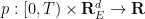
where is the velocity field and is the pressure field. These are functions of time and on the spatial location variable . We will refer to the coordinates as Eulerian coordinates. However, if one reviews the physical derivation of the Euler equations from 254A Notes 0, before one takes the continuum limit, the fundamental unknowns were not the velocity field or the pressure field , but rather the trajectories , which can be thought of as a single function from the coordinates (where is a time and is an element of the label set ) to . The relationship between the trajectories and the velocity field was given by the informal relationship

We will refer to the coordinates as (discrete) Lagrangian coordinates for describing the fluid.
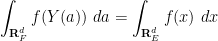
In view of this, it is natural to ask whether there is an alternate way to formulate the continuum limit of incompressible inviscid fluids, by using a continuous version of the Lagrangian coordinates, rather than Eulerian coordinates. This is indeed the case. Suppose for instance one has a smooth solution to the Euler equations on a spacetime slab in Eulerian coordinates; assume furthermore that the velocity field is uniformly bounded. We introduce another copy of , which we call Lagrangian space or labels space; we use symbols such as to refer to elements of this space, to denote Lebesgue measure on , and to refer to the coordinates of . We use indices such as to index these coordinates, thus for instance denotes partial differentiation along the coordinate. We will use summation conventions for both the Eulerian coordinates and the Lagrangian coordinates , with an index being summed if it appears as both a subscript and a superscript in the same term. While and are of course isomorphic, we will try to refrain from identifying them, except perhaps at the initial time in order to fix the initialisation of Lagrangian coordinates.
Given a smooth and bounded velocity field , define a trajectory map for this velocity to be any smooth map that obeys the ODE

in view of (2), this describes the trajectory (in ) of a particle labeled by an element of . From the Picard existence theorem and the hypothesis that is smooth and bounded, such a map exists and is unique as long as one specifies the initial location assigned to each label . Traditionally, one chooses the initial condition

for , so that we label each particle by its initial location at time ; we are also free to specify other initial conditions for the trajectory map if we please. Indeed, we have the freedom to “permute” the labels by an arbitrary diffeomorphism: if is a trajectory map, and is any diffeomorphism (a smooth map whose inverse exists and is also smooth), then the map is also a trajectory map, albeit one with different initial conditions .
Despite the popularity of the initial condition (4), we will try to keep conceptually separate the Eulerian space from the Lagrangian space , as they play different physical roles in the interpretation of the fluid; for instance, while the Euclidean metric is an important feature of Eulerian space , it is not a geometrically natural structure to use in Lagrangian space . We have the following more general version of Exercise 8 from 254A Notes 2:

Exercise 1 Let be smooth and bounded.

• If is a smooth map, show that there exists a unique smooth trajectory map with initial condition for all .
• Show that if is a diffeomorphism and , then the map is also a diffeomorphism.

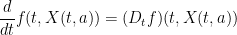
Remark 2 The first of the Euler equations (1) can now be written in the form

which can be viewed as a continuous limit of Newton’s first law .

Call a diffeomorphism (oriented) volume preserving if one has the equation

for all , where the total differential is the matrix with entries for and , where are the components of . (If one wishes, one can also view as a linear transformation from the tangent space of Lagrangian space at to the tangent space of Eulerian space at .) Equivalently, is orientation preserving and one has a Jacobian-free change of variables formula

for all , which is in turn equivalent to having the same Lebesgue measure as for any measurable set .
The divergence-free condition then can be nicely expressed in terms of volume-preserving properties of the trajectory maps , in a manner which confirms the interpretation of this condition as an incompressibility condition on the fluid:

Lemma 3 Let be smooth and bounded, let be a volume-preserving diffeomorphism, and let be the trajectory map. Then the following are equivalent:

• on .
• is volume-preserving for all .

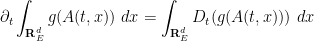
Proof: Since is orientation-preserving, we see from continuity that is also orientation-preserving. Suppose that is also volume-preserving, then for any we have the conservation law

for all . Differentiating in time using the chain rule and (3) we conclude that

for all , and hence by change of variables

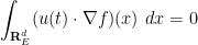
which by integration by parts gives

for all and , so is divergence-free.
To prove the converse implication, it is convenient to introduce the labels map , defined by setting to be the inverse of the diffeomorphism , thus

for all . By the implicit function theorem, is smooth, and by differentiating the above equation in time using (3) we see that

where is the usual material derivative

acting on functions on . If is divergence-free, we have from integration by parts that

for any test function . In particular, for any , we can calculate

and hence

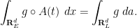
for any . Since is volume-preserving, so is , thus

Thus is volume-preserving, and hence is also.

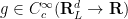
Exercise 4 Let be a continuously differentiable map from the time interval to the general linear group of invertible matrices. Establish Jacobi’s formula

and use this and (6) to give an alternate proof of Lemma 3 that does not involve any integration in space.

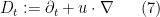
Remark 5 One can view the use of Lagrangian coordinates as an extension of the method of characteristics. Indeed, from the chain rule we see that for any smooth function of Eulerian spacetime, one has

and hence any transport equation that in Eulerian coordinates takes the form

for smooth functions of Eulerian spacetime is equivalent to the ODE

where are the smooth functions of Lagrangian spacetime defined by

In this set of notes we recall some basic differential geometry notation, particularly with regards to pullbacks and Lie derivatives of differential forms and other tensor fields on manifolds such as and , and explore how the Euler equations look in this notation. Our discussion will be entirely formal in nature; we will assume that all functions have enough smoothness and decay at infinity to justify the relevant calculations. (It is possible to work rigorously in Lagrangian coordinates – see for instance the work of Ebin and Marsden – but we will not do so here.) As a general rule, Lagrangian coordinates tend to be somewhat less convenient to use than Eulerian coordinates for establishing the basic analytic properties of the Euler equations, such as local existence, uniqueness, and continuous dependence on the data; however, they are quite good at clarifying the more algebraic properties of these equations, such as conservation laws and the variational nature of the equations. It may well be that in the future we will be able to use the Lagrangian formalism more effectively on the analytic side of the subject also.

Remark 6 One can also write the Navier-Stokes equations in Lagrangian coordinates, but the equations are not expressed in a favourable form in these coordinates, as the Laplacian appearing in the viscosity term becomes replaced with a time-varying Laplace-Beltrami operator. As such, we will not discuss the Lagrangian coordinate formulation of Navier-Stokes here.

246A, Notes 5: conformal mapping

Previous set of notes: Notes 4. Next set of notes: 246B Notes 1.
In the previous set of notes we introduced the notion of a complex diffeomorphism between two open subsets of the complex plane (or more generally, two Riemann surfaces): an invertible holomorphic map whose inverse was also holomorphic. (Actually, the last part is automatic, thanks to Exercise 41 of Notes 4.) Such maps are also known as biholomorphic maps or conformal maps (although in some literature the notion of “conformal map” is expanded to permit maps such as the complex conjugation map that are angle-preserving but not orientation-preserving, as well as maps such as the exponential map from to that are only locally injective rather than globally injective). Such complex diffeomorphisms can be used in complex analysis (or in the analysis of harmonic functions) to change the underlying domain to a domain that may be more convenient for calculations, thanks to the following basic lemma:

Lemma 1 (Holomorphicity and harmonicity are conformal invariants) Let be a complex diffeomorphism between two Riemann surfaces .

• (i) If is a function to another Riemann surface , then is holomorphic if and only if is holomorphic.
• (ii) If are open subsets of and is a function, then is harmonic if and only if is harmonic.

Proof: Part (i) is immediate since the composition of two holomorphic functions is holomorphic. For part (ii), observe that if is harmonic then on any ball in , is the real part of some holomorphic function thanks to Exercise 62 of Notes 3. By part (i), is also holomorphic. Taking real parts we see that is harmonic on each ball preimage in , and hence harmonic on all of , giving one direction of (ii); the other direction is proven similarly.

Exercise 2 Establish Lemma 1(ii) by direct calculation, avoiding the use of holomorphic functions. (Hint: the calculations are cleanest if one uses Wirtinger derivatives, as per Exercise 27 of Notes 1.)

Exercise 3 Let be a complex diffeomorphism between two open subsets of , let be a point in , let be a natural number, and let be holomorphic. Show that has a zero (resp. a pole) of order at if and only if has a zero (resp. a pole) of order at .

From Lemma 1(ii) we can now define the notion of a harmonic function on a Riemann surface ; such a function is harmonic if, for every coordinate chart in some atlas, the map is harmonic. Lemma 1(ii) ensures that this definition of harmonicity does not depend on the choice of atlas. Similarly, using Exercise 3 one can define what it means for a holomorphic map on a Riemann surface to have a pole or zero of a given order at a point , with the definition being independent of the choice of atlas; we can also identify such functions as equivalence classes of meromorphic functions in complete analogy with the case of meromorphic functions on domains . Finally, we can define the notion of an essential singularity of a holomorphic function at some isolated singularity in a Riemann surface as one that cannot be extended to a holomorphic function .
In view of Lemma 1, it is thus natural to ask which Riemann surfaces are complex diffeomorphic to each other, and more generally to understand the space of holomorphic maps from one given Riemann surface to another. We will initially focus attention on three important model Riemann surfaces:

• (i) (Elliptic model) The Riemann sphere ;
• (ii) (Parabolic model) The complex plane ; and
• (iii) (Hyperbolic model) The unit disk .

The designation of these model Riemann surfaces as elliptic, parabolic, and hyperbolic comes from Riemannian geometry, where it is natural to endow each of these surfaces with a constant curvature Riemannian metric which is positive, zero, or negative in the elliptic, parabolic, and hyperbolic cases respectively. However, we will not discuss Riemannian geometry further here.
All three model Riemann surfaces are simply connected, but none of them are complex diffeomorphic to any other; indeed, there are no non-constant holomorphic maps from the Riemann sphere to the plane or the disk, nor are there any non-constant holomorphic maps from the plane to the disk (although there are plenty of holomorphic maps going in the opposite directions). The complex automorphisms (that is, the complex diffeomorphisms from a surface to itself) of each of the three surfaces can be classified explicitly. The automorphisms of the Riemann sphere turn out to be the Möbius transformations with , also known as fractional linear transformations. The automorphisms of the complex plane are the linear transformations with , and the automorphisms of the disk are the fractional linear transformations of the form for and . Holomorphic maps from the disk to itself that fix the origin obey a basic but incredibly important estimate known as the Schwarz lemma: they are “dominated” by the identity function in the sense that for all . Among other things, this lemma gives guidance to determine when a given Riemann surface is complex diffeomorphic to a disk; we shall discuss this point further below.
It is a beautiful and fundamental fact in complex analysis that these three model Riemann surfaces are in fact an exhaustive list of the simply connected Riemann surfaces, up to complex diffeomorphism. More precisely, we have the Riemann mapping theorem and the uniformisation theorem:

Theorem 4 (Riemann mapping theorem) Let be a simply connected open subset of that is not all of . Then is complex diffeomorphic to .

Theorem 5 (Uniformisation theorem) Let be a simply connected Riemann surface. Then is complex diffeomorphic to , , or .

As we shall see, every connected Riemann surface can be viewed as the quotient of its simply connected universal cover by a discrete group of automorphisms known as deck transformations. This in principle gives a complete classification of Riemann surfaces up to complex diffeomorphism, although the situation is still somewhat complicated in the hyperbolic case because of the wide variety of discrete groups of automorphisms available in that case.
We will prove the Riemann mapping theorem in these notes, using the elegant argument of Koebe that is based on the Schwarz lemma and Montel’s theorem (Exercise 58 of Notes 4). The uniformisation theorem is however more difficult to establish; we discuss some components of a proof (based on the Perron method of subharmonic functions) here, but stop short of providing a complete proof.
The above theorems show that it is in principle possible to conformally map various domains into model domains such as the unit disk, but the proofs of these theorems do not readily produce explicit conformal maps for this purpose. For some domains we can just write down a suitable such map. For instance:

Exercise 6 (Cayley transform) Let be the upper half-plane. Show that the Cayley transform , defined by

is a complex diffeomorphism from the upper half-plane to the disk , with inverse map given by

Exercise 7 Show that for any real numbers , the strip is complex diffeomorphic to the disk . (Hint: use the complex exponential and a linear transformation to map the strip onto the half-plane .)

Exercise 8 Show that for any real numbers , the strip is complex diffeomorphic to the disk . (Hint: use a branch of either the complex logarithm, or of a complex power .)

We will discuss some other explicit conformal maps in this set of notes, such as the Schwarz-Christoffel maps that transform the upper half-plane to polygonal regions. Further examples of conformal mapping can be found in the text of Stein-Shakarchi.

Math 246A, Notes 4: singularities of holomorphic functions

Previous set of notes: Notes 3. Next set of notes: Notes 5.

In the previous set of notes we saw that functions that were holomorphic on an open set enjoyed a large number of useful properties, particularly if the domain was simply connected. In many situations, though, we need to consider functions that are only holomorphic (or even well-defined) on most of a domain , thus they are actually functions outside of some small singular set inside . (In this set of notes we only consider interior singularities; one can also discuss singular behaviour at the boundary of , but this is a whole separate topic and will not be pursued here.) Since we have only defined the notion of holomorphicity on open sets, we will require the singular sets to be closed, so that the domain on which remains holomorphic is still open. A typical class of examples are the functions of the form that were already encountered in the Cauchy integral formula; if is holomorphic and , such a function would be holomorphic save for a singularity at . Another basic class of examples are the rational functions , which are holomorphic outside of the zeroes of the denominator .

Singularities come in varying levels of “badness” in complex analysis. The least harmful type of singularity is the removable singularity – a point which is an isolated singularity (i.e., an isolated point of the singular set ) where the function is undefined, but for which one can extend the function across the singularity in such a fashion that the function becomes holomorphic in a neighbourhood of the singularity. A typical example is that of the complex sinc function , which has a removable singularity at the origin , which can be removed by declaring the sinc function to equal at . The detection of isolated removable singularities can be accomplished by Riemann’s theorem on removable singularities (Exercise 37 from Notes 3): if a holomorphic function is bounded near an isolated singularity , then the singularity at may be removed.

After removable singularities, the mildest form of singularity one can encounter is that of a pole – an isolated singularity such that can be factored as for some (known as the order of the pole), where has a removable singularity at (and is non-zero at once the singularity is removed). Such functions have already made a frequent appearance in previous notes, particularly the case of simple poles when . The behaviour near of function with a pole of order is well understood: for instance, goes to infinity as approaches (at a rate comparable to ). These singularities are not, strictly speaking, removable; but if one compactifies the range of the holomorphic function to a slightly larger space known as the Riemann sphere, then the singularity can be removed. In particular, functions which only have isolated singularities that are either poles or removable can be extended to holomorphic functions to the Riemann sphere. Such functions are known as meromorphic functions, and are nearly as well-behaved as holomorphic functions in many ways. In fact, in one key respect, the family of meromorphic functions is better: the meromorphic functions on turn out to form a field, in particular the quotient of two meromorphic functions is again meromorphic (if the denominator is not identically zero).

Unfortunately, there are isolated singularities that are neither removable or poles, and are known as essential singularities. A typical example is the function , which turns out to have an essential singularity at . The behaviour of such essential singularities is quite wild; we will show here the Casorati-Weierstrass theorem, which shows that the image of near the essential singularity is dense in the complex plane, as well as the more difficult great Picard theorem which asserts that in fact the image can omit at most one point in the complex plane. Nevertheless, around any isolated singularity (even the essential ones) , it is possible to expand as a variant of a Taylor series known as a Laurent series . The coefficient of this series is particularly important for contour integration purposes, and is known as the residue of at the isolated singularity . These residues play a central role in a common generalisation of Cauchy’s theorem and the Cauchy integral formula known as the residue theorem, which is a particularly useful tool for computing (or at least transforming) contour integrals of meromorphic functions, and has proven to be a particularly popular technique to use in analytic number theory. Within complex analysis, one important consequence of the residue theorem is the argument principle, which gives a topological (and analytical) way to control the zeroes and poles of a meromorphic function.

Finally, there are the non-isolated singularities. Little can be said about these singularities in general (for instance, the residue theorem does not directly apply in the presence of such singularities), but certain types of non-isolated singularities are still relatively easy to understand. One particularly common example of such non-isolated singularity arises when trying to invert a non-injective function, such as the complex exponential or a power function , leading to branches of multivalued functions such as the complex logarithm or the root function respectively. Such branches will typically have a non-isolated singularity along a branch cut; this branch cut can be moved around the complex domain by switching from one branch to another, but usually cannot be eliminated entirely, unless one is willing to lift up the domain to a more general type of domain known as a Riemann surface. As such, one can view branch cuts as being an “artificial” form of singularity, being an artefact of a choice of local coordinates of a Riemann surface, rather than reflecting any intrinsic singularity of the function itself. The further study of Riemann surfaces is an important topic in complex analysis (as well as the related fields of complex geometry and algebraic geometry), but this topic will be postponed to the next course in this sequence.

Notes on the Nash embedding theorem

Throughout this post we shall always work in the smooth category, thus all manifolds, maps, coordinate charts, and functions are assumed to be smooth unless explicitly stated otherwise.

A (real) manifold can be defined in at least two ways. On one hand, one can define the manifold extrinsically, as a subset of some standard space such as a Euclidean space . On the other hand, one can define the manifold intrinsically, as a topological space equipped with an atlas of coordinate charts. The fundamental embedding theorems show that, under reasonable assumptions, the intrinsic and extrinsic approaches give the same classes of manifolds (up to isomorphism in various categories). For instance, we have the following (special case of) the Whitney embedding theorem:

Theorem 1 (Whitney embedding theorem) Let be a compact manifold. Then there exists an embedding from to a Euclidean space .

In fact, if is -dimensional, one can take to equal , which is often best possible (easy examples include the circle which embeds into but not , or the Klein bottle that embeds into but not ). One can also relax the compactness hypothesis on to second countability, but we will not pursue this extension here. We give a “cheap” proof of this theorem below the fold which allows one to take equal to .

A significant strengthening of the Whitney embedding theorem is (a special case of) the Nash embedding theorem:

Theorem 2 (Nash embedding theorem) Let be a compact Riemannian manifold. Then there exists a isometric embedding from to a Euclidean space .

In order to obtain the isometric embedding, the dimension has to be a bit larger than what is needed for the Whitney embedding theorem; in this article of Gunther the bound

 

is attained, which I believe is still the record for large . (In the converse direction, one cannot do better than , basically because this is the number of degrees of freedom in the Riemannian metric .) Nash’s original proof of theorem used what is now known as Nash-Moser inverse function theorem, but a subsequent simplification of Gunther allowed one to proceed using just the ordinary inverse function theorem (in Banach spaces).

I recently had the need to invoke the Nash embedding theorem to establish a blowup result for a nonlinear wave equation, which motivated me to go through the proof of the theorem more carefully. Below the fold I give a proof of the theorem that does not attempt to give an optimal value of , but which hopefully isolates the main ideas of the argument (as simplified by Gunther). One advantage of not optimising in is that it allows one to freely exploit the very useful tool of pairing together two maps , to form a combined map that can be closer to an embedding or an isometric embedding than the original maps . This lets one perform a “divide and conquer” strategy in which one first starts with the simpler problem of constructing some “partial” embeddings of and then pairs them together to form a “better” embedding.

In preparing these notes, I found the articles of Deane Yang and of Siyuan Lu to be helpful.

Khot, Osher, Griffiths

In addition to the Fields medallists mentioned in the previous post, the IMU also awarded the Nevanlinna prize to Subhash Khot, the Gauss prize to Stan Osher (my colleague here at UCLA!), and the Chern medal to Phillip Griffiths. Like I did in 2010, I’ll try to briefly discuss one result of each of the prize winners, though the fields of mathematics here are even further from my expertise than those discussed in the previous post (and all the caveats from that post apply here also).

Subhash Khot is best known for his Unique Games Conjecture, a problem in complexity theory that is perhaps second in importance only to the problem for the purposes of demarcating the mysterious line between “easy” and “hard” problems (if one follows standard practice and uses “polynomial time” as the definition of “easy”). The problem can be viewed as an assertion that it is difficult to find exact solutions to certain standard theoretical computer science problems (such as -SAT); thanks to the NP-completeness phenomenon, it turns out that the precise problem posed here is not of critical importance, and -SAT may be substituted with one of the many other problems known to be NP-complete. The unique games conjecture is similarly an assertion about the difficulty of finding even approximate solutions to certain standard problems, in particular “unique games” problems in which one needs to colour the vertices of a graph in such a way that the colour of one vertex of an edge is determined uniquely (via a specified matching) by the colour of the other vertex. This is an easy problem to solve if one insists on exact solutions (in which 100% of the edges have a colouring compatible with the specified matching), but becomes extremely difficult if one permits approximate solutions, with no exact solution available. In analogy with the NP-completeness phenomenon, the threshold for approximate satisfiability of many other problems (such as the MAX-CUT problem) is closely connected with the truth of the unique games conjecture; remarkably, the truth of the unique games conjecture would imply asymptotically sharp thresholds for many of these problems. This has implications for many theoretical computer science constructions which rely on hardness of approximation, such as probabilistically checkable proofs. For a more detailed survey of the unique games conjecture and its implications, see this Bulletin article of Trevisan.

My colleague Stan Osher has worked in many areas of applied mathematics, ranging from image processing to modeling fluids for major animation studies such as Pixar or Dreamworks, but today I would like to talk about one of his contributions that is close to an area of my own expertise, namely compressed sensing. One of the basic reconstruction problem in compressed sensing is the basis pursuit problem of finding the vector in an affine space (where and are given, and is typically somewhat smaller than ) which minimises the -norm of the vector . This is a convex optimisation problem, and thus solvable in principle (it is a polynomial time problem, and thus “easy” in the above theoretical computer science sense). However, once and get moderately large (e.g. of the order of ), standard linear optimisation routines begin to become computationally expensive; also, it is difficult for off-the-shelf methods to exploit any additional structure (e.g. sparsity) in the measurement matrix . Much of the problem comes from the fact that the functional is only barely convex. One way to speed up the optimisation problem is to relax it by replacing the constraint with a convex penalty term , thus one is now trying to minimise the unconstrained functional

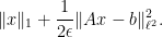
This functional is more convex, and is over a computationally simpler domain than the affine space , so is easier (though still not entirely trivial) to optimise over. However, the minimiser to this problem need not match the minimiser to the original problem, particularly if the (sub-)gradient of the original functional is large at , and if is not set to be small. (And setting too small will cause other difficulties with numerically solving the optimisation problem, due to the need to divide by very small denominators.) However, if one modifies the objective function by an additional linear term

then some simple convexity considerations reveal that the minimiser to this new problem will match the minimiser to the original problem, provided that is (or more precisely, lies in) the (sub-)gradient of at – even if is not small. But, one does not know in advance what the correct value of should be, because one does not know what the minimiser is.

With Yin, Goldfarb and Darbon, Osher introduced a Bregman iteration method in which one solves for and simultaneously; given an initial guess for both and , one first updates to the minimiser of the convex functional

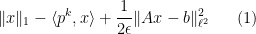
and then updates to the natural value of the subgradient at , namely

(note upon taking the first variation of (1) that is indeed in the subgradient). This procedure converges remarkably quickly (both in theory and in practice) to the true minimiser even for non-small values of , and also has some ability to be parallelised, and has led to actual performance improvements of an order of magnitude or more in certain compressed sensing problems (such as reconstructing an MRI image).

Phillip Griffiths has made many contributions to complex, algebraic and differential geometry, and I am not qualified to describe most of these; my primary exposure to his work is through his text on algebraic geometry with Harris, but as excellent though that text is, it is not really representative of his research. But I thought I would mention one cute result of his related to the famous Nash embedding theorem. Suppose that one has a smooth -dimensional Riemannian manifold that one wants to embed locally into a Euclidean space . The Nash embedding theorem guarantees that one can do this if is large enough depending on , but what is the minimal value of one can get away with? Many years ago, my colleague Robert Greene showed that sufficed (a simplified proof was subsequently given by Gunther). However, this is not believed to be sharp; if one replaces “smooth” with “real analytic” then a standard Cauchy-Kovalevski argument shows that is possible, and no better. So this suggests that is the threshold for the smooth problem also, but this remains open in general. The cases is trivial, and the case is not too difficult (if the curvature is non-zero) as the codimension is one in this case, and the problem reduces to that of solving a Monge-Ampere equation. With Bryant and Yang, Griffiths settled the case, under a non-degeneracy condition on the Einstein tensor. This is quite a serious paper – over 100 pages combining differential geometry, PDE methods (e.g. Nash-Moser iteration), and even some harmonic analysis (e.g. they rely at one key juncture on an extension theorem of my advisor, Elias Stein). The main difficulty is that that the relevant PDE degenerates along a certain characteristic submanifold of the cotangent bundle, which then requires an extremely delicate analysis to handle.

The Monge-Cayley-Salmon theorem via classical differential geometry

Let be an irreducible polynomial in three variables. As is not algebraically closed, the zero set can split into various components of dimension between and . For instance, if , the zero set is a line; more interestingly, if , then is the union of a line and a surface (or the product of an acnodal cubic curve with a line). We will assume that the -dimensional component is non-empty, thus defining a real surface in . In particular, this hypothesis implies that is not just irreducible over , but is in fact absolutely irreducible (i.e. irreducible over ), since otherwise one could use the complex factorisation of to contain inside the intersection of the complex zero locus of complex polynomial and its complex conjugate, with having no common factor, forcing to be at most one-dimensional. (For instance, in the case , one can take .) Among other things, this makes a Zariski-dense subset of , thus any polynomial identity which holds true at every point of , also holds true on all of . This allows us to easily use tools from algebraic geometry in this real setting, even though the reals are not quite algebraically closed.

The surface is said to be ruled if, for a Zariski open dense set of points , there exists a line through for some non-zero which is completely contained in , thus

for all . Also, a point is said to be a flecnode if there exists a line through for some non-zero which is tangent to to third order, in the sense that

as , or equivalently that

 

for . Clearly, if is a ruled surface, then a Zariski open dense set of points on are a flecnode. We then have the remarkable theorem (discovered first by Monge, and then later by Cayley and Salmon) asserting the converse:

Theorem 1 (Monge-Cayley-Salmon theorem) Let be an irreducible polynomial with non-empty. Suppose that a Zariski dense set of points in are flecnodes. Then is a ruled surface.

Among other things, this theorem was used in the celebrated result of Guth and Katz that almost solved the Erdos distance problem in two dimensions, as discussed in this previous blog post. Vanishing to third order is necessary: observe that in a surface of negative curvature, such as the saddle , every point on the surface is tangent to second order to a line (the line in the direction for which the second fundamental form vanishes). This surface happens to be ruled, but a generic perturbation of this surface (e.g. ) will no longer be ruled, although it is still negative curvature near the origin.

The original proof of the Monge-Cayley-Salmon theorem is not easily accessible and not written in modern language. A modern proof of this theorem (together with substantial generalisations, for instance to higher dimensions) is given by Landsberg; the proof uses the machinery of modern algebraic geometry. The purpose of this post is to record an alternate proof of the Monge-Cayley-Salmon theorem based on classical differential geometry (in particular, the notion of torsion of a curve) and basic ODE methods (in particular, Gronwall’s inequality and the Picard existence theorem). The idea is to “integrate” the lines indicated by the flecnode to produce smooth curves on the surface ; one then uses the vanishing (1) and some basic calculus to conclude that these curves have zero torsion and are thus planar curves. Some further manipulation using (1) (now just to second order instead of third) then shows that these curves are in fact straight lines, giving the ruling on the surface.

Update: Janos Kollar has informed me that the above theorem was essentially known to Monge in 1809; see his recent arXiv note for more details.

I thank Larry Guth and Micha Sharir for conversations leading to this post.

254A, Notes 1: Lie groups, Lie algebras, and the Baker-Campbell-Hausdorff formula

In this set of notes, we describe the basic analytic structure theory of Lie groups, by relating them to the simpler concept of a Lie algebra. Roughly speaking, the Lie algebra encodes the “infinitesimal” structure of a Lie group, but is a simpler object, being a vector space rather than a nonlinear manifold. Nevertheless, thanks to the fundamental theorems of Lie, the Lie algebra can be used to reconstruct the Lie group (at a local level, at least), by means of the exponential map and the Baker-Campbell-Hausdorff formula. As such, the local theory of Lie groups is completely described (in principle, at least) by the theory of Lie algebras, which leads to a number of useful consequences, such as the following:

• (Local Lie implies Lie) A topological group is Lie (i.e. it is isomorphic to a Lie group) if and only if it is locally Lie (i.e. the group operations are smooth near the origin).
• (Uniqueness of Lie structure) A topological group has at most one smooth structure on it that makes it Lie.
• (Weak regularity implies strong regularity, I) Lie groups are automatically real analytic. (In fact one only needs a “local ” regularity on the group structure to obtain real analyticity.)
• (Weak regularity implies strong regularity, II) A continuous homomorphism from one Lie group to another is automatically smooth (and real analytic).

The connection between Lie groups and Lie algebras also highlights the role of one-parameter subgroups of a topological group, which will play a central role in the solution of Hilbert’s fifth problem.

We note that there is also a very important algebraic structure theory of Lie groups and Lie algebras, in which the Lie algebra is split into solvable and semisimple components, with the latter being decomposed further into simple components, which can then be completely classified using Dynkin diagrams. This classification is of fundamental importance in many areas of mathematics (e.g. representation theory, arithmetic geometry, and group theory), and many of the deeper facts about Lie groups and Lie algebras are proven via this classification (although in such cases it can be of interest to also find alternate proofs that avoid the classification). However, it turns out that we will not need this theory in this course, and so we will not discuss it further here (though it can of course be found in any graduate text on Lie groups and Lie algebras).

Two small facts about Lie groups

Over the past few months or so, I have been brushing up on my Lie group theory, as part of my project to fully understand the theory surrounding Hilbert’s fifth problem. Every so often, I encounter a basic fact in Lie theory which requires a slightly non-trivial “trick” to prove; I am recording two of them here, so that I can find these tricks again when I need to.

The first fact concerns the exponential map from a Lie algebra of a Lie group to that group. (For this discussion we will only consider finite-dimensional Lie groups and Lie algebras over the reals .) A basic fact in the subject is that the exponential map is locally a homeomorphism: there is a neighbourhood of the origin in that is mapped homeomorphically by the exponential map to a neighbourhood of the identity in . This local homeomorphism property is the foundation of an important dictionary between Lie groups and Lie algebras.

It is natural to ask whether the exponential map is globally a homeomorphism, and not just locally: in particular, whether the exponential map remains both injective and surjective. For instance, this is the case for connected, simply connected, nilpotent Lie groups (as can be seen from the Baker-Campbell-Hausdorff formula.)

The circle group , which has as its Lie algebra, already shows that global injectivity fails for any group that contains a circle subgroup, which is a huge class of examples (including, for instance, the positive dimensional compact Lie groups, or non-simply-connected Lie groups). Surjectivity also obviously fails for disconnected groups, since the Lie algebra is necessarily connected, and so the image under the exponential map must be connected also. However, even for connected Lie groups, surjectivity can fail. To see this, first observe that if the exponential map was surjective, then every group element has a square root (i.e. an element with ), since has as a square root for any . However, there exist elements in connected Lie groups without square roots. A simple example is provided by the matrix

in the connected Lie group . This matrix has eigenvalues , . Thus, if is a square root of , we see (from the Jordan normal form) that it must have at least one eigenvalue in , and at least one eigenvalue in . On the other hand, as has real coefficients, the complex eigenvalues must come in conjugate pairs . Since can only have at most eigenvalues, we obtain a contradiction.

However, there is an important case where surjectivity is recovered:

Proposition 1 If is a compact connected Lie group, then the exponential map is surjective.

Proof: The idea here is to relate the exponential map in Lie theory to the exponential map in Riemannian geometry. We first observe that every compact Lie group can be given the structure of a Riemannian manifold with a bi-invariant metric. This can be seen in one of two ways. Firstly, one can put an arbitrary positive definite inner product on and average it against the adjoint action of using Haar probability measure (which is available since is compact); this gives an ad-invariant positive-definite inner product on that one can then translate by either left or right translation to give a bi-invariant Riemannian structure on . Alternatively, one can use the Peter-Weyl theorem to embed in a unitary group , at which point one can induce a bi-invariant metric on from the one on the space of complex matrices.

As is connected and compact and thus complete, we can apply the Hopf-Rinow theorem and conclude that any two points are connected by at least one geodesic, so that the Riemannian exponential map from to formed by following geodesics from the origin is surjective. But one can check that the Lie exponential map and Riemannian exponential map agree; for instance, this can be seen by noting that the group structure naturally defines a connection on the tangent bundle which is both torsion-free and preserves the bi-invariant metric, and must therefore agree with the Levi-Civita metric. (Alternatively, one can embed into a unitary group and observe that is totally geodesic inside , because the geodesics in can be described explicitly in terms of one-parameter subgroups.) The claim follows.

Remark 1 While it is quite nice to see Riemannian geometry come in to prove this proposition, I am curious to know if there is any other proof of surjectivity for compact connected Lie groups that does not require explicit introduction of Riemannian geometry concepts.

The other basic fact I learned recently concerns the algebraic nature of Lie groups and Lie algebras. An important family of examples of Lie groups are the algebraic groups – algebraic varieties with a group law given by algebraic maps. Given that one can always automatically upgrade the smooth structure on a Lie group to analytic structure (by using the Baker-Campbell-Hausdorff formula), it is natural to ask whether one can upgrade the structure further to an algebraic structure. Unfortunately, this is not always the case. A prototypical example of this is given by the one-parameter subgroup

of . This is a Lie group for any exponent , but if is irrational, then the curve that traces out is not an algebraic subset of (as one can see by playing around with Puiseux series).

This is not a true counterexample to the claim that every Lie group can be given the structure of an algebraic group, because one can give a different algebraic structure than one inherited from the ambient group . Indeed, is clearly isomorphic to the additive group , which is of course an algebraic group. However, a modification of the above construction works:

Proposition 2 There exists a Lie group that cannot be given the structure of an algebraic group.

Proof: We use an example from the text of Tauvel and Yu (that I found via this MathOverflow posting). We consider the subgroup

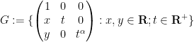
of , with an irrational number. This is a three-dimensional (metabelian) Lie group, whose Lie algebra is spanned by the elements

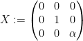
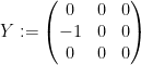
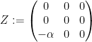
with the Lie bracket given by

As such, we see that if we use the basis to identify to , then adjoint representation of is the identity map.

If is an algebraic group, it is easy to see that the adjoint representation is also algebraic, and so is algebraic in . Specialising to our specific example, in which adjoint representation is the identity, we conclude that if has any algebraic structure, then it must also be an algebraic subgroup of ; but projects to the group (1) which is not algebraic, a contradiction.

A slight modification of the same argument also shows that not every Lie algebra is algebraic, in the sense that it is isomorphic to a Lie algebra of an algebraic group. (However, there are important classes of Lie algebras that are automatically algebraic, such as nilpotent or semisimple Lie algebras.)

Hilbert’s fifth problem and Gleason metrics

Hilbert’s fifth problem asks to clarify the extent that the assumption on a differentiable or smooth structure is actually needed in the theory of Lie groups and their actions. While this question is not precisely formulated and is thus open to some interpretation, the following result of Gleason and Montgomery-Zippin answers at least one aspect of this question:

Theorem 1 (Hilbert’s fifth problem) Let be a topological group which is locally Euclidean (i.e. it is a topological manifold). Then is isomorphic to a Lie group.

Theorem 1 can be viewed as an application of the more general structural theory of locally compact groups. In particular, Theorem 1 can be deduced from the following structural theorem of Gleason and Yamabe:

Theorem 2 (Gleason-Yamabe theorem) Let be a locally compact group, and let be an open neighbourhood of the identity in . Then there exists an open subgroup of , and a compact subgroup of contained in , such that is isomorphic to a Lie group.

The deduction of Theorem 1 from Theorem 2 proceeds using the Brouwer invariance of domain theorem and is discussed in this previous post. In this post, I would like to discuss the proof of Theorem 2. We can split this proof into three parts, by introducing two additional concepts. The first is the property of having no small subgroups:

Definition 3 (NSS) A topological group is said to have no small subgroups, or is NSS for short, if there is an open neighbourhood of the identity in that contains no subgroups of other than the trivial subgroup .

An equivalent definition of an NSS group is one which has an open neighbourhood of the identity that every non-identity element escapes in finite time, in the sense that for some positive integer . It is easy to see that all Lie groups are NSS; we shall shortly see that the converse statement (in the locally compact case) is also true, though significantly harder to prove.

Another useful property is that of having what I will call a Gleason metric:

Definition 4 Let be a topological group. A Gleason metric on is a left-invariant metric which generates the topology on and obeys the following properties for some constant , writing for :

• (Escape property) If and is such that , then .
• (Commutator estimate) If are such that , then

  

  where is the commutator of and .

For instance, the unitary group with the operator norm metric can easily verified to be a Gleason metric, with the commutator estimate (1) coming from the inequality

Similarly, any left-invariant Riemannian metric on a (connected) Lie group can be verified to be a Gleason metric. From the escape property one easily sees that all groups with Gleason metrics are NSS; again, we shall see that there is a partial converse.

Remark 1 The escape and commutator properties are meant to capture “Euclidean-like” structure of the group. Other metrics, such as Carnot-Carathéodory metrics on Carnot Lie groups such as the Heisenberg group, usually fail one or both of these properties.

The proof of Theorem 2 can then be split into three subtheorems:

Theorem 5 (Reduction to the NSS case) Let be a locally compact group, and let be an open neighbourhood of the identity in . Then there exists an open subgroup of , and a compact subgroup of contained in , such that is NSS, locally compact, and metrisable.

Theorem 6 (Gleason’s lemma) Let be a locally compact metrisable NSS group. Then has a Gleason metric.

Theorem 7 (Building a Lie structure) Let be a locally compact group with a Gleason metric. Then is isomorphic to a Lie group.

Clearly, by combining Theorem 5, Theorem 6, and Theorem 7 one obtains Theorem 2 (and hence Theorem 1).

Theorem 5 and Theorem 6 proceed by some elementary combinatorial analysis, together with the use of Haar measure (to build convolutions, and thence to build “smooth” bump functions with which to create a metric, in a variant of the analysis used to prove the Birkhoff-Kakutani theorem); Theorem 5 also requires Peter-Weyl theorem (to dispose of certain compact subgroups that arise en route to the reduction to the NSS case), which was discussed previously on this blog.

In this post I would like to detail the final component to the proof of Theorem 2, namely Theorem 7. (I plan to discuss the other two steps, Theorem 5 and Theorem 6, in a separate post.) The strategy is similar to that used to prove von Neumann’s theorem, as discussed in this previous post (and von Neumann’s theorem is also used in the proof), but with the Gleason metric serving as a substitute for the faithful linear representation. Namely, one first gives the space of one-parameter subgroups of enough of a structure that it can serve as a proxy for the “Lie algebra” of ; specifically, it needs to be a vector space, and the “exponential map” needs to cover an open neighbourhood of the identity. This is enough to set up an “adjoint” representation of , whose image is a Lie group by von Neumann’s theorem; the kernel is essentially the centre of , which is abelian and can also be shown to be a Lie group by a similar analysis. To finish the job one needs to use arguments of Kuranishi and of Gleason, as discussed in this previous post.

The arguments here can be phrased either in the standard analysis setting (using sequences, and passing to subsequences often) or in the nonstandard analysis setting (selecting an ultrafilter, and then working with infinitesimals). In my view, the two approaches have roughly the same level of complexity in this case, and I have elected for the standard analysis approach.

Remark 2 From Theorem 7 we see that a Gleason metric structure is a good enough substitute for smooth structure that it can actually be used to reconstruct the entire smooth structure; roughly speaking, the commutator estimate (1) allows for enough “Taylor expansion” of expressions such as that one can simulate the fundamentals of Lie theory (in particular, construction of the Lie algebra and the exponential map, and its basic properties. The advantage of working with a Gleason metric rather than a smoother structure, though, is that it is relatively undemanding with regards to regularity; in particular, the commutator estimate (1) is roughly comparable to the imposition structure on the group , as this is the minimal regularity to get the type of Taylor approximation (with quadratic errors) that would be needed to obtain a bound of the form (1). We will return to this point in a later post.