
You are currently browsing the category archive for the ‘math.AP’ category.
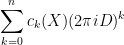
Marcel Filoche, Svitlana Mayboroda, and I have just uploaded to the arXiv our preprint “The effective potential of an 


Suppose one has an eigenfunction

 , where
  is the Laplacian on
  ,
,  is a potential, and
  is an energy. Where would one expect the eigenfunction
  to be concentrated? If the potential
  is smooth and slowly varying, the correspondence principle suggests that the eigenfunction should be mostly concentrated in the potential energy wells
  , with an exponentially decaying amount of tunnelling between the wells. One way to rigorously establish such an exponential decay is through an argument of Agmon, which we will sketch later in this post, which gives an exponentially decaying upper bound (in an
  sense) of eigenfunctions in terms of the distance to the wells
  in terms of a certain “Agmon metric” on determined by the potential and energy level (or any upper bound
  on this energy). Similar exponential decay results can also be obtained for discrete Schrödinger matrix models, in which the domain is replaced with a discrete set such as the lattice
  , and the Laplacian is replaced by a discrete analogue such as a graph Laplacian.
When the potential 


There are now several explanations for why this particular choice 


These particular explanations seem rather specific to the Schrödinger equation (continuous or discrete); we have for instance not been able to find similar identities to explain an effective potential for the bi-Schrödinger operator 
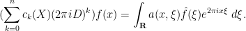
In this paper, we demonstrate the (perhaps surprising) fact that effective potentials continue to exist for operators that bear very little resemblance to Schrödinger operators. Our chosen model is that of an 


 is normalised in
  , where the connectivity
  is the maximum number of non-zero entries of in any row or column,
  are the coefficients of , and
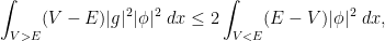
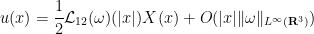
  is a certain moderately complicated but explicit metric function on the spatial domain. Informally, this inequality asserts that the eigenfunction
  should decay like
  or faster. Indeed, our numerics show a very strong log-linear relationship between and
  , although it appears that our exponent
  is not quite optimal. We also provide an associated localisation result which is technical to state but very roughly asserts that a given eigenvector will in fact be localised to a single connected component of
  unless there is a resonance between two wells (by which we mean that an eigenvalue for a localisation of associated to one well is extremely close to an eigenvalue for a localisation of associated to another well); such localisation is also strongly supported by numerics. (Analogous results for Schrödinger operators had been previously obtained by the previously mentioned paper of Arnold, David, Jerison, and my two coauthors, and to quantum graphs in a very recent paper of Harrell and Maltsev.)
Our approach is based on Agmon’s methods, which we interpret as a double commutator method, and in particular relying on exploiting the negative definiteness of certain double commutator operators. In the case of Schrödinger operators 

![\displaystyle \langle [[-\Delta+V,g],g] u, u \rangle = -2\int_{{\bf R}^d} |\nabla g|^2 |u|^2\ dx \leq 0 \ \ \ \ \ (2)](https://s0.wp.com/latex.php?latex=%5Cdisplaystyle++%5Clangle+%5B%5B-%5CDelta%2BV%2Cg%5D%2Cg%5D+u%2C+u+%5Crangle+%3D+-2%5Cint_%7B%7B%5Cbf+R%7D%5Ed%7D+%7C%5Cnabla+g%7C%5E2+%7Cu%7C%5E2%5C+dx+%5Cleq+0+%5C+%5C+%5C+%5C+%5C+%282%29&bg=ffffff&fg=000000&s=0&c=20201002)
![\displaystyle \langle g [\psi, -\Delta+V] u, g \psi u \rangle = \frac{1}{2} \langle [[-\Delta+V, g \psi],g\psi] u, u \rangle](https://s0.wp.com/latex.php?latex=%5Cdisplaystyle++%5Clangle+g+%5B%5Cpsi%2C+-%5CDelta%2BV%5D+u%2C+g+%5Cpsi+u+%5Crangle+%3D+%5Cfrac%7B1%7D%7B2%7D+%5Clangle+%5B%5B-%5CDelta%2BV%2C+g+%5Cpsi%5D%2Cg%5Cpsi%5D+u%2C+u+%5Crangle+&bg=ffffff&fg=000000&s=0&c=20201002)
![\displaystyle -\frac{1}{2} \langle [[-\Delta+V, g],g] \psi u, \psi u \rangle](https://s0.wp.com/latex.php?latex=%5Cdisplaystyle+-%5Cfrac%7B1%7D%7B2%7D+%5Clangle+%5B%5B-%5CDelta%2BV%2C+g%5D%2Cg%5D+%5Cpsi+u%2C+%5Cpsi+u+%5Crangle+&bg=ffffff&fg=000000&s=0&c=20201002)
 after a brief calculation. The double commutator identity then tells us that
 ![\displaystyle \langle g [\psi, -\Delta+V] u, g \psi u \rangle \leq \int_{{\bf R}^d} |\nabla g|^2 |\psi u|^2\ dx.](https://s0.wp.com/latex.php?latex=%5Cdisplaystyle++%5Clangle+g+%5B%5Cpsi%2C+-%5CDelta%2BV%5D+u%2C+g+%5Cpsi+u+%5Crangle+%5Cleq+%5Cint_%7B%7B%5Cbf+R%7D%5Ed%7D+%7C%5Cnabla+g%7C%5E2+%7C%5Cpsi+u%7C%5E2%5C+dx.&bg=ffffff&fg=000000&s=0&c=20201002) to be a non-negative weight and let
to be a non-negative weight and let  for an eigenfunction , then we can write
 ![\displaystyle [\psi, -\Delta+V] u = [\psi, -\Delta+V - E] u = \psi (-\Delta+V - E) u](https://s0.wp.com/latex.php?latex=%5Cdisplaystyle++%5B%5Cpsi%2C+-%5CDelta%2BV%5D+u+%3D+%5B%5Cpsi%2C+-%5CDelta%2BV+-+E%5D+u+%3D+%5Cpsi+%28-%5CDelta%2BV+-+E%29+u&bg=ffffff&fg=000000&s=0&c=20201002)

 . If we select
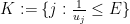
  , we obtain the clean inequality
  to be a function which equals on the wells but increases exponentially away from these wells, in such a way that
 away from the wells. This is basically the classic exponential decay estimate of Agmon; one can basically take to be the distance to the wells with respect to the Euclidean metric conformally weighted by a suitably normalised version of
  . If we instead select to be the landscape function
 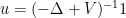 , (3) then gives
  appropriately this gives an exponential decay estimate away from the effective wells
  , using a metric weighted by
  .
.
It turns out that this argument extends without much difficulty to the
![\displaystyle \langle [[A,D],D] u, u \rangle = \sum_{i \neq j} a_{ij} u_i u_j (d_{ii} - d_{jj})^2 \leq 0](https://s0.wp.com/latex.php?latex=%5Cdisplaystyle++%5Clangle+%5B%5BA%2CD%5D%2CD%5D+u%2C+u+%5Crangle%09%3D+%5Csum_%7Bi+%5Cneq+j%7D+a_%7Bij%7D+u_i+u_j+%28d_%7Bii%7D+-+d_%7Bjj%7D%29%5E2+%5Cleq+0&bg=ffffff&fg=000000&s=0&c=20201002)
 . The remainder of the Agmon type arguments go through after making the natural modifications.
Numerically we have also found some aspects of the landscape theory to persist beyond the
In contrast to previous notes, in this set of notes we shall focus exclusively on Fourier analysis in the one-dimensional setting 

In previous notes we have often performed various localisations in either physical space or Fourier space 
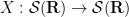
and the momentum operator 
(The terminology comes from quantum mechanics, where it is customary to also insert a small constant 


for any 


for all 

Clearly, for any polynomial 


and similarly the operator 
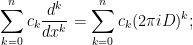
Inspired by this, if 
for all 


one can easily verify from several applications of the Leibniz rule that 


For instance, any constant coefficient linear differential operators 
however there are many Fourier multiplier operators that are not of this form, such as fractional derivative operators 


We observe that the maps 


and

for any 


for 
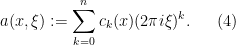
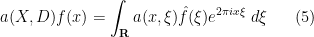
In the field of PDE and ODE, it is also very common to study variable coefficient linear differential operators
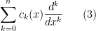
where the 

and so it is natural to interpret this operator as a combination 


Indeed, from the Fourier inversion formula
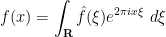
for any
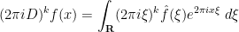
and hence on multiplying by 
Inspired by this, we can introduce the Kohn-Nirenberg quantisation by defining the operator 
whenever
for all 


 are two functions obeying
  for all
  . (Hint: apply
  to a suitable truncation of a plane wave
  and then take limits.)
In principle, the quantisations 

in general. Fundamentally, this is due to the fact that pointwise multiplication of symbols is a commutative operation, whereas the composition of operators such as
![\displaystyle [A,B] := AB - BA](https://s0.wp.com/latex.php?latex=%5Cdisplaystyle++%5BA%2CB%5D+%3A%3D+AB+-+BA&bg=ffffff&fg=000000&s=0&c=20201002)
of two operators 
![\displaystyle [X,D] = -\frac{1}{2\pi i} \neq 0.](https://s0.wp.com/latex.php?latex=%5Cdisplaystyle++%5BX%2CD%5D+%3D+-%5Cfrac%7B1%7D%7B2%5Cpi+i%7D+%5Cneq+0.&bg=ffffff&fg=000000&s=0&c=20201002)
(In the language of Lie groups and Lie algebras, this tells us that
Exercise 2 (Heisenberg uncertainty principle) For any
and
, show that
(Hint: evaluate the expression
in two different ways and apply the Cauchy-Schwarz inequality.) Informally, this exercise asserts that the spatial uncertainty
and the frequency uncertainty
of a function obey the Heisenberg uncertainty relation
.

Nevertheless, one still has the correspondence principle, which asserts that in certain regimes (which, with our choice of normalisations, corresponds to the high-frequency regime), quantum mechanics continues to behave like a commutative theory, and one can sometimes proceed as if the operators

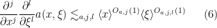
where the error between the left and right-hand sides is of “lower order” and can in fact enjoys a useful asymptotic expansion. As a first approximation to this calculus, one can think of functions 


Unfortunately the uncertainty principle (or the non-commutativity of 
To complement the pseudodifferential calculus we have the basic Calderón-Vaillancourt theorem, which asserts that pseudodifferential operators of order zero are Calderón-Zygmund operators and thus bounded on 

Pseudodifferential operators (especially when generalised to higher dimensions 
This set of notes is only the briefest introduction to the theory of pseudodifferential operators. Many texts are available that cover the theory in more detail, for instance this text of Taylor.
Just a brief post to record some notable papers in my fields of interest that appeared on the arXiv recently.
- “A sharp square function estimate for the cone in
“, by Larry Guth, Hong Wang, and Ruixiang Zhang. This paper establishes an optimal (up to epsilon losses) square function estimate for the three-dimensional light cone that was essentially conjectured by Mockenhaupt, Seeger, and Sogge, which has a number of other consequences including Sogge’s local smoothing conjecture for the wave equation in two spatial dimensions, which in turn implies the (already known) Bochner-Riesz, restriction, and Kakeya conjectures in two dimensions. Interestingly, modern techniques such as polynomial partitioning and decoupling estimates are not used in this argument; instead, the authors mostly rely on an induction on scales argument and Kakeya type estimates. Many previous authors (including myself) were able to get weaker estimates of this type by an induction on scales method, but there were always significant inefficiencies in doing so; in particular knowing the sharp square function estimate at smaller scales did not imply the sharp square function estimate at the given larger scale. The authors here get around this issue by finding an even stronger estimate that implies the square function estimate, but behaves significantly better with respect to induction on scales.
- “On the Chowla and twin primes conjectures over
“, by Will Sawin and Mark Shusterman. This paper resolves a number of well known open conjectures in analytic number theory, such as the Chowla conjecture and the twin prime conjecture (in the strong form conjectured by Hardy and Littlewood), in the case of function fields where the field is a prime power
which is fixed (in contrast to a number of existing results in the “large
” limit) but has a large exponent
. The techniques here are orthogonal to those used in recent progress towards the Chowla conjecture over the integers (e.g., in this previous paper of mine); the starting point is an algebraic observation that in certain function fields, the Mobius function behaves like a quadratic Dirichlet character along certain arithmetic progressions. In principle, this reduces problems such as Chowla’s conjecture to problems about estimating sums of Dirichlet characters, for which more is known; but the task is still far from trivial.
- “Bounds for sets with no polynomial progressions“, by Sarah Peluse. This paper can be viewed as part of a larger project to obtain quantitative density Ramsey theorems of Szemeredi type. For instance, Gowers famously established a relatively good quantitative bound for Szemeredi’s theorem that all dense subsets of integers contain arbitrarily long arithmetic progressions
. The corresponding question for polynomial progressions
is considered more difficult for a number of reasons. One of them is that dilation invariance is lost; a dilation of an arithmetic progression is again an arithmetic progression, but a dilation of a polynomial progression will in general not be a polynomial progression with the same polynomials
. Another issue is that the ranges of the two parameters
are now at different scales. Peluse gets around these difficulties in the case when all the polynomials
, so that one can still run a density increment argument efficiently. To resolve the second difficulty one needs to find a quantitative concatenation theorem for Gowers uniformity norms. Many of these ideas were developed in previous papers of Peluse and Peluse-Prendiville in simpler settings.
- “On blow up for the energy super critical defocusing non linear Schrödinger equations“, by Frank Merle, Pierre Raphael, Igor Rodnianski, and Jeremie Szeftel. This paper (when combined with two companion papers) resolves a long-standing problem as to whether finite time blowup occurs for the defocusing supercritical nonlinear Schrödinger equation (at least in certain dimensions and nonlinearities). I had a previous paper establishing a result like this if one “cheated” by replacing the nonlinear Schrodinger equation by a system of such equations, but remarkably they are able to tackle the original equation itself without any such cheating. Given the very analogous situation with Navier-Stokes, where again one can create finite time blowup by “cheating” and modifying the equation, it does raise hope that finite time blowup for the incompressible Navier-Stokes and Euler equations can be established… In fact the connection may not just be at the level of analogy; a surprising key ingredient in the proofs here is the observation that a certain blowup ansatz for the nonlinear Schrodinger equation is governed by solutions to the (compressible) Euler equation, and finite time blowup examples for the latter can be used to construct finite time blowup examples for the former.
Let 


(From a differential geometry viewpoint, it would be more accurate (especially in other dimensions than three) to define the vorticity as the exterior derivative 

Assuming suitable regularity and decay hypotheses of the velocity field 

and thus (by the commutativity of all the differential operators involved)

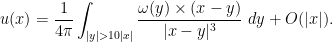
Using the Newton potential formula

and formally differentiating under the integral sign, we obtain the Biot-Savart law

This law is of fundamental importance in the study of incompressible fluid equations, such as the Euler equations

since on applying the curl operator one obtains the vorticity equation

and then by substituting (1) one gets an autonomous equation for the vorticity field 
In a recent work, it was observed by Elgindi that in a certain regime, the Biot-Savart law can be approximated by a more “low rank” law, which makes the non-local effects significantly simpler in nature. This simplification was carried out in spherical coordinates, and hinged on a study of the invertibility properties of a certain second order linear differential operator in the latitude variable 
Elgindi’s approximation applies under the following hypotheses:
- (i) (Axial symmetry without swirl) The velocity field
for some functionsof the cylindrical radial variable
and the vertical coordinate
. As a consequence, the vorticity field
whereis the field
- (ii) (Odd symmetry) We assume that
and
, so that
.


A model example of a divergence-free vector field obeying these properties (but without good decay at infinity) is the linear vector field

which is of the form (3) with 

We can now give an illustration of Elgindi’s approximation:
Proposition 1 (Elgindi’s approximation) Under the above hypotheses (and assuing suitable regularity and decay), we have the pointwise bounds
for any
, where
is the scalar function

Thus under the hypotheses (i), (ii), and assuming that 

then we have (using the spherical change of variables formula 


where
is the operator introduced in Elgindi’s paper.
Proof: By a limiting argument we may assume that 


and hence by (1)
In the regime 


Since
we see from the triangle inequality that the error term contributes 


where 

and 

By the hypotheses (i), (ii), we have the symmetries


The even symmetry (8) ensures that the integrand in 


Using (4), the right-hand side is


where 


Using the rotation symmetry 


giving the claim.

Example 2 Consider the divergence-free vector field
, where the vector potential
for some bump function
supported in
. We can then calculate
and
In particular the hypotheses (i), (ii) are satisfied with
One can then calculate
If we take the specific choice
where
is a fixed bump function supported some interval
and
is a small parameter (so that
is spread out over the range
), then we see that
(with implied constants allowed to depend on
and
which is completely consistent with Proposition 1.


One can use this approximation to extract a plausible ansatz for a self-similar blowup to the Euler equations. We let 

where 


By Proposition 1, we thus expect to have the approximation

We insert this into the vorticity equation (2). The transport term 


and so in the limit 
If we write 


which integrates to the Ricatti equation

which can be explicitly solved as

where 


and then on applying 
Thus, we expect to be able to construct a self-similar blowup to the Euler equations with a vorticity field approximately behaving like

and velocity field behaving like

In particular, 


and

A self-similar solution of this approximate shape is in fact constructed rigorously in Elgindi’s paper (using spherical coordinates instead of the Cartesian approach adopted here), using a nonlinear stability analysis of the above ansatz. It seems plausible that one could also carry out this stability analysis using this Cartesian coordinate approach, although I have not tried to do this in detail.
I’ve just uploaded to the arXiv my paper “Quantitative bounds for critically bounded solutions to the Navier-Stokes equations“, submitted to the proceedings of the Linde Hall Inaugural Math Symposium. (I unfortunately had to cancel my physical attendance at this symposium for personal reasons, but was still able to contribute to the proceedings.) In recent years I have been interested in working towards establishing the existence of classical solutions for the Navier-Stokes equations


that blow up in finite time, but this time for a change I took a look at the other side of the theory, namely the conditional regularity results for this equation. There are several such results that assert that if a certain norm of the solution stays bounded (or grows at a controlled rate), then the solution stays regular; taken in the contrapositive, they assert that if a solution blows up at a certain finite time 
- (Leray blowup criterion, 1934) If
, then
for an absolute constant
.
- (Prodi–Serrin–Ladyzhenskaya blowup criterion, 1959-1967) If
, where
.
- (Beale-Kato-Majda blowup criterion, 1984) If
, where
is the vorticity.
- (Kato blowup criterion, 1984) If
for some absolute constant
- (Escauriaza-Seregin-Sverak blowup criterion, 2003) If
.
- (Seregin blowup criterion, 2012) If
.
- (Phuc blowup criterion, 2015) If
for any
.
- (Gallagher-Koch-Planchon blowup criterion, 2016) If
for any
.
- (Albritton blowup criterion, 2016) If
for any
My current paper is most closely related to the Escauriaza-Seregin-Sverak blowup criterion, which was the first to show a critical (i.e., scale-invariant, or dimensionless) spatial norm, namely 

On the other hand, it is a general principle that qualitative arguments established using compactness methods ought to have quantitative analogues that replace the use of compactness by more complicated substitutes that give effective bounds; see for instance these previous blog posts for more discussion. I therefore was interested in trying to obtain a quantitative version of this blowup criterion that gave reasonably good effective bounds (in particular, my objective was to avoid truly enormous bounds such as tower-exponential or Ackermann function bounds, which often arise if one “naively” tries to make a compactness argument effective). In particular, I obtained the following triple-exponential quantitative regularity bounds:
Theorem 1 If
with
and
for
and
.

 , then

As a corollary, one can now improve the Escauriaza-Seregin-Sverak blowup criterion to
for some absolute constant
The proof uses many of the same quantitative inputs as previous arguments, most notably the Carleman inequalities used to establish unique continuation and backwards uniqueness theorems for backwards heat equations, but also some additional techniques that make the quantitative bounds more efficient. The proof focuses initially on points of concentration of the solution, which we define as points 


for a large absolute constant 


from which the above theorem ends up following from a routine adaptation of the local well-posedness and regularity theory for Navier-Stokes.
The strategy is to show that any concentration such as (2) when 


- Firstly, by using Duhamel’s formula, one can show that a concentration (2) can only occur (with
at some slightly previous point
in spacetime, with
also close to
,
, and
). This can be viewed as a sort of contrapositive of a “local regularity theorem”, such as the ones established by Caffarelli, Kohn, and Nirenberg. A key point here is that the lower bound
in the conclusion (3) is precisely the same as the lower bound in (2), so that this backwards propagation of concentration can be iterated.
- Iterating the previous step, one can find a sequence of concentration points
with the
propagating backwards in time; by using estimates ultimately resulting from the dissipative term in the energy identity, one can extract such a sequence in which the
increase geometrically with time, the
are comparable (up to polynomial factors in
, and one has
. Using the “epochs of regularity” theory that ultimately dates back to Leray, and tweaking the
slightly, one can also place the times
(of length comparable to a small multiple of
) in which the solution is quite regular (in particular,
enjoy good
bounds on
).
- The concentration (4) can be used to establish a lower bound for the
norm of the vorticity
In the epoch of regularity
of this equation obey good
bounds, allowing the machinery of Carleman estimates to come into play. Using a Carleman estimate that is used to establish unique continuation results for backwards heat equations, one can propagate this lower bound to also give lower
for various radii
, although the lower bounds decay at a gaussian rate with
- Meanwhile, using an energy pigeonholing argument of Bourgain (which, in this Navier-Stokes context, is actually an enstrophy pigeonholing argument), one can locate some annuli
where (a slightly normalised form of) the entrosphy is small at time
; using a version of the localised enstrophy estimates from a previous paper of mine, one can then propagate this sort of control forward in time, obtaining an “annulus of regularity” of the form
in which one has good estimates; in particular, one has
- By intersecting the previous epoch of regularity
, establishing a lower bound for the vorticity on the spatial annulus
. By some basic Littlewood-Paley theory one can parlay this lower bound to a lower bound on the
norm of the velocity
.
- If


The chain of causality is summarised in the following image:

It seems natural to conjecture that similar triply logarithmic improvements can be made to several of the other blowup criteria listed above, but I have not attempted to pursue this question. It seems difficult to improve the triple logarithmic factor using only the techniques here; the Bourgain pigeonholing argument inevitably costs one exponential, the Carleman inequalities cost a second, and the stacking of scales at the end to contradict the
Let 


for any permutation 


will be an element of 


Given two natural numbers 

![{[F^{(k)}]_{k \rightarrow p} \in L(\Omega^p)_{sym}}](https://s0.wp.com/latex.php?latex=%7B%5BF%5E%7B%28k%29%7D%5D_%7Bk+%5Crightarrow+p%7D+%5Cin+L%28%5COmega%5Ep%29_%7Bsym%7D%7D&bg=ffffff&fg=000000&s=0&c=20201002)
![\displaystyle [F^{(k)}]_{k \rightarrow p}(x_1,\dots,x_p) = \sum_{1 \leq i_1 < i_2 < \dots < i_k \leq p} F^{(k)}(x_{i_1}, \dots, x_{i_k})](https://s0.wp.com/latex.php?latex=%5Cdisplaystyle+%5BF%5E%7B%28k%29%7D%5D_%7Bk+%5Crightarrow+p%7D%28x_1%2C%5Cdots%2Cx_p%29+%3D+%5Csum_%7B1+%5Cleq+i_1+%3C+i_2+%3C+%5Cdots+%3C+i_k+%5Cleq+p%7D+F%5E%7B%28k%29%7D%28x_%7Bi_1%7D%2C+%5Cdots%2C+x_%7Bi_k%7D%29+&bg=ffffff&fg=000000&s=0&c=20201002)
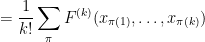
where 


![{[F^{(k)}]_{k \rightarrow p}}](https://s0.wp.com/latex.php?latex=%7B%5BF%5E%7B%28k%29%7D%5D_%7Bk+%5Crightarrow+p%7D%7D&bg=ffffff&fg=000000&s=0&c=20201002)
![\displaystyle [F^{(1)}(x_1)]_{1 \rightarrow p} = \sum_{i=1}^p F^{(1)}(x_i)](https://s0.wp.com/latex.php?latex=%5Cdisplaystyle+%5BF%5E%7B%281%29%7D%28x_1%29%5D_%7B1+%5Crightarrow+p%7D+%3D+%5Csum_%7Bi%3D1%7D%5Ep+F%5E%7B%281%29%7D%28x_i%29&bg=ffffff&fg=000000&s=0&c=20201002)
![\displaystyle [F^{(2)}(x_1,x_2)]_{2 \rightarrow p} = \sum_{1 \leq i < j \leq p} F^{(2)}(x_i,x_j)](https://s0.wp.com/latex.php?latex=%5Cdisplaystyle+%5BF%5E%7B%282%29%7D%28x_1%2Cx_2%29%5D_%7B2+%5Crightarrow+p%7D+%3D+%5Csum_%7B1+%5Cleq+i+%3C+j+%5Cleq+p%7D+F%5E%7B%282%29%7D%28x_i%2Cx_j%29&bg=ffffff&fg=000000&s=0&c=20201002)
and
![\displaystyle e_k^{(p)}(x_1,\dots,x_p) = [x_1 \dots x_k]_{k \rightarrow p}.](https://s0.wp.com/latex.php?latex=%5Cdisplaystyle+e_k%5E%7B%28p%29%7D%28x_1%2C%5Cdots%2Cx_p%29+%3D+%5Bx_1+%5Cdots+x_k%5D_%7Bk+%5Crightarrow+p%7D.&bg=ffffff&fg=000000&s=0&c=20201002)
Also we have
![\displaystyle [1]_{k \rightarrow p} = \binom{p}{k} = \frac{p(p-1)\dots(p-k+1)}{k!}.](https://s0.wp.com/latex.php?latex=%5Cdisplaystyle+%5B1%5D_%7Bk+%5Crightarrow+p%7D+%3D+%5Cbinom%7Bp%7D%7Bk%7D+%3D+%5Cfrac%7Bp%28p-1%29%5Cdots%28p-k%2B1%29%7D%7Bk%21%7D.&bg=ffffff&fg=000000&s=0&c=20201002)
With these conventions, we see that 


![\displaystyle [F^{(k)}]_{k \rightarrow p} = \frac{1}{\binom{p-k}{p-l}} [[F^{(k)}]_{k \rightarrow l}]_{l \rightarrow p}](https://s0.wp.com/latex.php?latex=%5Cdisplaystyle+%5BF%5E%7B%28k%29%7D%5D_%7Bk+%5Crightarrow+p%7D+%3D+%5Cfrac%7B1%7D%7B%5Cbinom%7Bp-k%7D%7Bp-l%7D%7D+%5B%5BF%5E%7B%28k%29%7D%5D_%7Bk+%5Crightarrow+l%7D%5D_%7Bl+%5Crightarrow+p%7D&bg=ffffff&fg=000000&s=0&c=20201002)
if 
The lifting map ![{[]_{k \rightarrow p}}](https://s0.wp.com/latex.php?latex=%7B%5B%5D_%7Bk+%5Crightarrow+p%7D%7D&bg=ffffff&fg=000000&s=0&c=20201002)


![\displaystyle [x_1]_{1 \rightarrow p} [x_1]_{1 \rightarrow p} = (\sum_{i=1}^p x_i)^2 \ \ \ \ \ (1)](https://s0.wp.com/latex.php?latex=%5Cdisplaystyle+%5Bx_1%5D_%7B1+%5Crightarrow+p%7D+%5Bx_1%5D_%7B1+%5Crightarrow+p%7D+%3D+%28%5Csum_%7Bi%3D1%7D%5Ep+x_i%29%5E2+%5C+%5C+%5C+%5C+%5C+%281%29&bg=ffffff&fg=000000&s=0&c=20201002)
![\displaystyle = [x_1^2]_{1 \rightarrow p} + 2 [x_1 x_2]_{1 \rightarrow p}](https://s0.wp.com/latex.php?latex=%5Cdisplaystyle+%3D+%5Bx_1%5E2%5D_%7B1+%5Crightarrow+p%7D+%2B+2+%5Bx_1+x_2%5D_%7B1+%5Crightarrow+p%7D&bg=ffffff&fg=000000&s=0&c=20201002)
![\displaystyle \neq [x_1^2]_{1 \rightarrow p}.](https://s0.wp.com/latex.php?latex=%5Cdisplaystyle+%5Cneq+%5Bx_1%5E2%5D_%7B1+%5Crightarrow+p%7D.&bg=ffffff&fg=000000&s=0&c=20201002)
In general, one has the identity
![\displaystyle [F^{(k)}(x_1,\dots,x_k)]_{k \rightarrow p} [G^{(l)}(x_1,\dots,x_l)]_{l \rightarrow p} = \sum_{k,l \leq m \leq k+l} \frac{1}{k! l!} \ \ \ \ \ (2)](https://s0.wp.com/latex.php?latex=%5Cdisplaystyle+%5BF%5E%7B%28k%29%7D%28x_1%2C%5Cdots%2Cx_k%29%5D_%7Bk+%5Crightarrow+p%7D+%5BG%5E%7B%28l%29%7D%28x_1%2C%5Cdots%2Cx_l%29%5D_%7Bl+%5Crightarrow+p%7D+%3D+%5Csum_%7Bk%2Cl+%5Cleq+m+%5Cleq+k%2Bl%7D+%5Cfrac%7B1%7D%7Bk%21+l%21%7D+%5C+%5C+%5C+%5C+%5C+%282%29&bg=ffffff&fg=000000&s=0&c=20201002)
![\displaystyle [\sum_{\pi, \rho} F^{(k)}(x_{\pi(1)},\dots,x_{\pi(k)}) G^{(l)}(x_{\rho(1)},\dots,x_{\rho(l)})]_{m \rightarrow p}](https://s0.wp.com/latex.php?latex=%5Cdisplaystyle+%5B%5Csum_%7B%5Cpi%2C+%5Crho%7D+F%5E%7B%28k%29%7D%28x_%7B%5Cpi%281%29%7D%2C%5Cdots%2Cx_%7B%5Cpi%28k%29%7D%29+G%5E%7B%28l%29%7D%28x_%7B%5Crho%281%29%7D%2C%5Cdots%2Cx_%7B%5Crho%28l%29%7D%29%5D_%7Bm+%5Crightarrow+p%7D&bg=ffffff&fg=000000&s=0&c=20201002)
for all natural numbers 


Example 1 When
, one has
which is just a restatement of the identity
![\displaystyle [x_1 x_2]_{2 \rightarrow p} [x_1]_{1 \rightarrow p} = [\frac{1}{2! 1!}( 2 x_1^2 x_2 + 2 x_1 x_2^2 )]_{2 \rightarrow p} + [\frac{1}{2! 1!} 6 x_1 x_2 x_3]_{3 \rightarrow p}](https://s0.wp.com/latex.php?latex=%5Cdisplaystyle+%5Bx_1+x_2%5D_%7B2+%5Crightarrow+p%7D+%5Bx_1%5D_%7B1+%5Crightarrow+p%7D+%3D+%5B%5Cfrac%7B1%7D%7B2%21+1%21%7D%28+2+x_1%5E2+x_2+%2B+2+x_1+x_2%5E2+%29%5D_%7B2+%5Crightarrow+p%7D+%2B+%5B%5Cfrac%7B1%7D%7B2%21+1%21%7D+6+x_1+x_2+x_3%5D_%7B3+%5Crightarrow+p%7D&bg=ffffff&fg=000000&s=0&c=20201002)
![\displaystyle = [x_1^2 x_2 + x_1 x_2^2]_{2 \rightarrow p} + [3x_1 x_2 x_3]_{3 \rightarrow p}](https://s0.wp.com/latex.php?latex=%5Cdisplaystyle+%3D+%5Bx_1%5E2+x_2+%2B+x_1+x_2%5E2%5D_%7B2+%5Crightarrow+p%7D+%2B+%5B3x_1+x_2+x_3%5D_%7B3+%5Crightarrow+p%7D&bg=ffffff&fg=000000&s=0&c=20201002)

Note that the coefficients appearing in (2) do not depend on the final number of variables 
![\displaystyle F^{(*)} = \sum_{k=0}^\infty [F^{(k)}]_{k \rightarrow *}](https://s0.wp.com/latex.php?latex=%5Cdisplaystyle+F%5E%7B%28%2A%29%7D+%3D+%5Csum_%7Bk%3D0%7D%5E%5Cinfty+%5BF%5E%7B%28k%29%7D%5D_%7Bk+%5Crightarrow+%2A%7D&bg=ffffff&fg=000000&s=0&c=20201002)
where for each 
![{[]_{k \rightarrow *}}](https://s0.wp.com/latex.php?latex=%7B%5B%5D_%7Bk+%5Crightarrow+%2A%7D%7D&bg=ffffff&fg=000000&s=0&c=20201002)
![\displaystyle [F^{(k)}]_{k \rightarrow *} + [G^{(k)}]_{k \rightarrow *} := [F^{(k)} + G^{(k)}]_{k \rightarrow *}](https://s0.wp.com/latex.php?latex=%5Cdisplaystyle+%5BF%5E%7B%28k%29%7D%5D_%7Bk+%5Crightarrow+%2A%7D+%2B+%5BG%5E%7B%28k%29%7D%5D_%7Bk+%5Crightarrow+%2A%7D+%3A%3D+%5BF%5E%7B%28k%29%7D+%2B+G%5E%7B%28k%29%7D%5D_%7Bk+%5Crightarrow+%2A%7D&bg=ffffff&fg=000000&s=0&c=20201002)
and
![\displaystyle c [F^{(k)}]_{k \rightarrow *} := [cF^{(k)}]_{k \rightarrow *}](https://s0.wp.com/latex.php?latex=%5Cdisplaystyle+c+%5BF%5E%7B%28k%29%7D%5D_%7Bk+%5Crightarrow+%2A%7D+%3A%3D+%5BcF%5E%7B%28k%29%7D%5D_%7Bk+%5Crightarrow+%2A%7D&bg=ffffff&fg=000000&s=0&c=20201002)
for 

![\displaystyle [F^{(k)}(x_1,\dots,x_k)]_{k \rightarrow *} [G^{(l)}(x_1,\dots,x_l)]_{l \rightarrow *} = \sum_{k,l \leq m \leq k+l} \frac{1}{k! l!} \ \ \ \ \ (3)](https://s0.wp.com/latex.php?latex=%5Cdisplaystyle+%5BF%5E%7B%28k%29%7D%28x_1%2C%5Cdots%2Cx_k%29%5D_%7Bk+%5Crightarrow+%2A%7D+%5BG%5E%7B%28l%29%7D%28x_1%2C%5Cdots%2Cx_l%29%5D_%7Bl+%5Crightarrow+%2A%7D+%3D+%5Csum_%7Bk%2Cl+%5Cleq+m+%5Cleq+k%2Bl%7D+%5Cfrac%7B1%7D%7Bk%21+l%21%7D+%5C+%5C+%5C+%5C+%5C+%283%29&bg=ffffff&fg=000000&s=0&c=20201002)
![\displaystyle [\sum_{\pi, \rho} F^{(k)}(x_{\pi(1)},\dots,x_{\pi(k)}) G^{(l)}(x_{\rho(1)},\dots,x_{\rho(l)})]_{m \rightarrow *}](https://s0.wp.com/latex.php?latex=%5Cdisplaystyle+%5B%5Csum_%7B%5Cpi%2C+%5Crho%7D+F%5E%7B%28k%29%7D%28x_%7B%5Cpi%281%29%7D%2C%5Cdots%2Cx_%7B%5Cpi%28k%29%7D%29+G%5E%7B%28l%29%7D%28x_%7B%5Crho%281%29%7D%2C%5Cdots%2Cx_%7B%5Crho%28l%29%7D%29%5D_%7Bm+%5Crightarrow+%2A%7D+&bg=ffffff&fg=000000&s=0&c=20201002)
of (2). Thus for instance, in this algebra
![\displaystyle [x_1]_{1 \rightarrow *} [x_1]_{1 \rightarrow *} = [x_1^2]_{1 \rightarrow *} + 2 [x_1 x_2]_{2 \rightarrow *}](https://s0.wp.com/latex.php?latex=%5Cdisplaystyle+%5Bx_1%5D_%7B1+%5Crightarrow+%2A%7D+%5Bx_1%5D_%7B1+%5Crightarrow+%2A%7D+%3D+%5Bx_1%5E2%5D_%7B1+%5Crightarrow+%2A%7D+%2B+2+%5Bx_1+x_2%5D_%7B2+%5Crightarrow+%2A%7D&bg=ffffff&fg=000000&s=0&c=20201002)
and
![\displaystyle [x_1 x_2]_{2 \rightarrow *} [x_1]_{1 \rightarrow *} = [x_1^2 x_2 + x_1 x_2^2]_{2 \rightarrow *} + [3 x_1 x_2 x_3]_{3 \rightarrow *}.](https://s0.wp.com/latex.php?latex=%5Cdisplaystyle+%5Bx_1+x_2%5D_%7B2+%5Crightarrow+%2A%7D+%5Bx_1%5D_%7B1+%5Crightarrow+%2A%7D+%3D+%5Bx_1%5E2+x_2+%2B+x_1+x_2%5E2%5D_%7B2+%5Crightarrow+%2A%7D+%2B+%5B3+x_1+x_2+x_3%5D_%7B3+%5Crightarrow+%2A%7D.&bg=ffffff&fg=000000&s=0&c=20201002)
Informally, ![{[1]_{0 \rightarrow *}}](https://s0.wp.com/latex.php?latex=%7B%5B1%5D_%7B0+%5Crightarrow+%2A%7D%7D&bg=ffffff&fg=000000&s=0&c=20201002)
For natural numbers ![{[]_{* \rightarrow p}}](https://s0.wp.com/latex.php?latex=%7B%5B%5D_%7B%2A+%5Crightarrow+p%7D%7D&bg=ffffff&fg=000000&s=0&c=20201002)
![\displaystyle [\sum_{k=0}^\infty [F^{(k)}]_{k \rightarrow *}]_{* \rightarrow p} := \sum_{k=0}^\infty [F^{(k)}]_{k \rightarrow p}.](https://s0.wp.com/latex.php?latex=%5Cdisplaystyle+%5B%5Csum_%7Bk%3D0%7D%5E%5Cinfty+%5BF%5E%7B%28k%29%7D%5D_%7Bk+%5Crightarrow+%2A%7D%5D_%7B%2A+%5Crightarrow+p%7D+%3A%3D+%5Csum_%7Bk%3D0%7D%5E%5Cinfty+%5BF%5E%7B%28k%29%7D%5D_%7Bk+%5Crightarrow+p%7D.&bg=ffffff&fg=000000&s=0&c=20201002)
Thus, for instance, ![{[x_1]_{1 \rightarrow *}}](https://s0.wp.com/latex.php?latex=%7B%5Bx_1%5D_%7B1+%5Crightarrow+%2A%7D%7D&bg=ffffff&fg=000000&s=0&c=20201002)
![{[x_1]_{1 \rightarrow p}}](https://s0.wp.com/latex.php?latex=%7B%5Bx_1%5D_%7B1+%5Crightarrow+p%7D%7D&bg=ffffff&fg=000000&s=0&c=20201002)
![{[x_1 x_2]_{2 \rightarrow *}}](https://s0.wp.com/latex.php?latex=%7B%5Bx_1+x_2%5D_%7B2+%5Crightarrow+%2A%7D%7D&bg=ffffff&fg=000000&s=0&c=20201002)
![{[x_1 x_2]_{2 \rightarrow p}}](https://s0.wp.com/latex.php?latex=%7B%5Bx_1+x_2%5D_%7B2+%5Crightarrow+p%7D%7D&bg=ffffff&fg=000000&s=0&c=20201002)
![{[]_{* \rightarrow p}: L(\Omega^*)_{sym} \rightarrow L(\Omega^p)_{sym}}](https://s0.wp.com/latex.php?latex=%7B%5B%5D_%7B%2A+%5Crightarrow+p%7D%3A+L%28%5COmega%5E%2A%29_%7Bsym%7D+%5Crightarrow+L%28%5COmega%5Ep%29_%7Bsym%7D%7D&bg=ffffff&fg=000000&s=0&c=20201002)
![{[]_{k \rightarrow *}: L(\Omega^k)_{sym} \rightarrow L(\Omega^*)_{sym}}](https://s0.wp.com/latex.php?latex=%7B%5B%5D_%7Bk+%5Crightarrow+%2A%7D%3A+L%28%5COmega%5Ek%29_%7Bsym%7D+%5Crightarrow+L%28%5COmega%5E%2A%29_%7Bsym%7D%7D&bg=ffffff&fg=000000&s=0&c=20201002)
![{[]_{k \rightarrow p}: L(\Omega^k)_{sym} \rightarrow L(\Omega^p)_{sym}}](https://s0.wp.com/latex.php?latex=%7B%5B%5D_%7Bk+%5Crightarrow+p%7D%3A+L%28%5COmega%5Ek%29_%7Bsym%7D+%5Crightarrow+L%28%5COmega%5Ep%29_%7Bsym%7D%7D&bg=ffffff&fg=000000&s=0&c=20201002)

Now suppose that we have a measure 


In the event that
![\displaystyle \int_{{\bf R}^p} [x_1]_{1 \rightarrow p}\ d\mu^p = p (\int_{\bf R} x\ d\mu(x)) (\int_{\bf R} \mu)^{p-1} \ \ \ \ \ (4)](https://s0.wp.com/latex.php?latex=%5Cdisplaystyle+%5Cint_%7B%7B%5Cbf+R%7D%5Ep%7D+%5Bx_1%5D_%7B1+%5Crightarrow+p%7D%5C+d%5Cmu%5Ep+%3D+p+%28%5Cint_%7B%5Cbf+R%7D+x%5C+d%5Cmu%28x%29%29+%28%5Cint_%7B%5Cbf+R%7D+%5Cmu%29%5E%7Bp-1%7D+%5C+%5C+%5C+%5C+%5C+%284%29&bg=ffffff&fg=000000&s=0&c=20201002)
![\displaystyle \int_{{\bf R}^p} [x_1 x_2]_{2 \rightarrow p}\ d\mu^p = \binom{p}{2} (\int_{{\bf R}^2} x_1 x_2\ d\mu(x_1) d\mu(x_2)) (\int_{\bf R} \mu)^{p-2}. \ \ \ \ \ (5)](https://s0.wp.com/latex.php?latex=%5Cdisplaystyle+%5Cint_%7B%7B%5Cbf+R%7D%5Ep%7D+%5Bx_1+x_2%5D_%7B2+%5Crightarrow+p%7D%5C+d%5Cmu%5Ep+%3D+%5Cbinom%7Bp%7D%7B2%7D+%28%5Cint_%7B%7B%5Cbf+R%7D%5E2%7D+x_1+x_2%5C+d%5Cmu%28x_1%29+d%5Cmu%28x_2%29%29+%28%5Cint_%7B%5Cbf+R%7D+%5Cmu%29%5E%7Bp-2%7D.+%5C+%5C+%5C+%5C+%5C+%285%29&bg=ffffff&fg=000000&s=0&c=20201002)
is an element of the formal algebra
![\displaystyle \int_{\Omega^p} [F^{(*)}]_{* \rightarrow p}\ d\mu^p = \sum_{k=0}^\infty \binom{p}{k} (\int_{\Omega^k} F^{(k)}\ d\mu^k) (\int_\Omega\ d\mu)^{p-k}. \ \ \ \ \ (6)](https://s0.wp.com/latex.php?latex=%5Cdisplaystyle+%5Cint_%7B%5COmega%5Ep%7D+%5BF%5E%7B%28%2A%29%7D%5D_%7B%2A+%5Crightarrow+p%7D%5C+d%5Cmu%5Ep+%3D+%5Csum_%7Bk%3D0%7D%5E%5Cinfty+%5Cbinom%7Bp%7D%7Bk%7D+%28%5Cint_%7B%5COmega%5Ek%7D+F%5E%7B%28k%29%7D%5C+d%5Cmu%5Ek%29+%28%5Cint_%5COmega%5C+d%5Cmu%29%5E%7Bp-k%7D.+%5C+%5C+%5C+%5C+%5C+%286%29&bg=ffffff&fg=000000&s=0&c=20201002)
Note that by hypothesis, only finitely many terms on the right-hand side are non-zero.
Now for a key observation: whereas the left-hand side of (6) only makes sense when 

![\displaystyle F^{(p)} = [F^{(*)}]_{* \rightarrow p} = \sum_{k=0}^\infty [F^{(k)}]_{k \rightarrow p}](https://s0.wp.com/latex.php?latex=%5Cdisplaystyle+F%5E%7B%28p%29%7D+%3D+%5BF%5E%7B%28%2A%29%7D%5D_%7B%2A+%5Crightarrow+p%7D+%3D+%5Csum_%7Bk%3D0%7D%5E%5Cinfty+%5BF%5E%7B%28k%29%7D%5D_%7Bk+%5Crightarrow+p%7D&bg=ffffff&fg=000000&s=0&c=20201002)
with 
![\displaystyle [F^{(*)}]_{* \rightarrow p} + [G^{(*)}]_{* \rightarrow p} := [F^{(*)} + G^{(*)}]_{* \rightarrow p}](https://s0.wp.com/latex.php?latex=%5Cdisplaystyle+%5BF%5E%7B%28%2A%29%7D%5D_%7B%2A+%5Crightarrow+p%7D+%2B+%5BG%5E%7B%28%2A%29%7D%5D_%7B%2A+%5Crightarrow+p%7D+%3A%3D+%5BF%5E%7B%28%2A%29%7D+%2B+G%5E%7B%28%2A%29%7D%5D_%7B%2A+%5Crightarrow+p%7D&bg=ffffff&fg=000000&s=0&c=20201002)
![\displaystyle c [F^{(*)}]_{* \rightarrow p} := [c F^{(*)}]_{* \rightarrow p}](https://s0.wp.com/latex.php?latex=%5Cdisplaystyle+c+%5BF%5E%7B%28%2A%29%7D%5D_%7B%2A+%5Crightarrow+p%7D+%3A%3D+%5Bc+F%5E%7B%28%2A%29%7D%5D_%7B%2A+%5Crightarrow+p%7D&bg=ffffff&fg=000000&s=0&c=20201002)
![\displaystyle [F^{(*)}]_{* \rightarrow p} [G^{(*)}]_{* \rightarrow p} := [F^{(*)} G^{(*)}]_{* \rightarrow p}.](https://s0.wp.com/latex.php?latex=%5Cdisplaystyle+%5BF%5E%7B%28%2A%29%7D%5D_%7B%2A+%5Crightarrow+p%7D+%5BG%5E%7B%28%2A%29%7D%5D_%7B%2A+%5Crightarrow+p%7D+%3A%3D+%5BF%5E%7B%28%2A%29%7D+G%5E%7B%28%2A%29%7D%5D_%7B%2A+%5Crightarrow+p%7D.&bg=ffffff&fg=000000&s=0&c=20201002)
In particular, the multiplication law (2) continues to hold for such values of 

Example 2 Suppose
is a random variable; on any power
, we let
be the usual independent copies of
for
. Then for any real or complex
can be evaluated by first using the identity
(cf. (1)) and then using (6) and the probability measure hypothesis
to conclude that
For
whenever
are jointly independent copies of
has expectation
and variance
. One can thus view (7) as an abstract generalisation of (8) to the case when
In this particular case, the quantity (7) is non-negative for every nonnegative
and the right-hand side can become negative for
. This is a shame, because otherwise one could hope to start endowing
with some sort of commutative von Neumann algebra type structure (or the abstract probability structure discussed in this previous post) and then interpret it as a genuine measure space rather than as a virtual one. (This failure of positivity is related to the fact that the characteristic function of a random variable, when raised to the
is non-negative, then so is
![\displaystyle \int_{\Omega^p} [X_1]_{1 \rightarrow p}^2\ d\mu^p](https://s0.wp.com/latex.php?latex=%5Cdisplaystyle+%5Cint_%7B%5COmega%5Ep%7D+%5BX_1%5D_%7B1+%5Crightarrow+p%7D%5E2%5C+d%5Cmu%5Ep+&bg=ffffff&fg=000000&s=0&c=20201002)
![\displaystyle [X_1]_{1 \rightarrow p}^2 = [X_1^2]_{1 \rightarrow p} + 2[X_1 X_2]_{2 \rightarrow p}](https://s0.wp.com/latex.php?latex=%5Cdisplaystyle+%5BX_1%5D_%7B1+%5Crightarrow+p%7D%5E2+%3D+%5BX_1%5E2%5D_%7B1+%5Crightarrow+p%7D+%2B+2%5BX_1+X_2%5D_%7B2+%5Crightarrow+p%7D&bg=ffffff&fg=000000&s=0&c=20201002)
![\displaystyle \int_{\Omega^p} [X_1]_{1 \rightarrow p}^2\ d\mu^p = \binom{p}{1} \int_{\Omega} X^2\ d\mu + 2 \binom{p}{2} \int_{\Omega^2} X_1 X_2\ d\mu^2](https://s0.wp.com/latex.php?latex=%5Cdisplaystyle+%5Cint_%7B%5COmega%5Ep%7D+%5BX_1%5D_%7B1+%5Crightarrow+p%7D%5E2%5C+d%5Cmu%5Ep+%3D+%5Cbinom%7Bp%7D%7B1%7D+%5Cint_%7B%5COmega%7D+X%5E2%5C+d%5Cmu+%2B+2+%5Cbinom%7Bp%7D%7B2%7D+%5Cint_%7B%5COmega%5E2%7D+X_1+X_2%5C+d%5Cmu%5E2&bg=ffffff&fg=000000&s=0&c=20201002)

![\displaystyle \int_{\Omega^p} [X_1]_{1 \rightarrow p}^2\ d\mu^p = p \mathbf{Var}(X) + p^2 \mathbf{E}(X)^2. \ \ \ \ \ (7)](https://s0.wp.com/latex.php?latex=%5Cdisplaystyle+%5Cint_%7B%5COmega%5Ep%7D+%5BX_1%5D_%7B1+%5Crightarrow+p%7D%5E2%5C+d%5Cmu%5Ep+%3D+p+%5Cmathbf%7BVar%7D%28X%29+%2B+p%5E2+%5Cmathbf%7BE%7D%28X%29%5E2.+%5C+%5C+%5C+%5C+%5C+%287%29&bg=ffffff&fg=000000&s=0&c=20201002)

![\displaystyle \int_{\Omega^p} [X_1]_{1 \rightarrow p}^4\ d\mu^p = p \mathbf{Var}(X^2) + p(3p-2) (\mathbf{E}(X^2))^2](https://s0.wp.com/latex.php?latex=%5Cdisplaystyle+%5Cint_%7B%5COmega%5Ep%7D+%5BX_1%5D_%7B1+%5Crightarrow+p%7D%5E4%5C+d%5Cmu%5Ep+%3D+p+%5Cmathbf%7BVar%7D%28X%5E2%29+%2B+p%283p-2%29+%28%5Cmathbf%7BE%7D%28X%5E2%29%29%5E2&bg=ffffff&fg=000000&s=0&c=20201002)
![\displaystyle \int_{\Omega^p} [F]_{1 \rightarrow p}\ d\mu^p = p (\int_\Omega F\ d\mu) (\int_\Omega\ d\mu)^{p-1}.](https://s0.wp.com/latex.php?latex=%5Cdisplaystyle+%5Cint_%7B%5COmega%5Ep%7D+%5BF%5D_%7B1+%5Crightarrow+p%7D%5C+d%5Cmu%5Ep+%3D+p+%28%5Cint_%5COmega+F%5C+d%5Cmu%29+%28%5Cint_%5COmega%5C+d%5Cmu%29%5E%7Bp-1%7D.&bg=ffffff&fg=000000&s=0&c=20201002)
One can wonder what the point is to all of this abstract formalism and how it relates to the rest of mathematics. For me, this formalism originated implicitly in an old paper I wrote with Jon Bennett and Tony Carbery on the multilinear restriction and Kakeya conjectures, though we did not have a good language for working with it at the time, instead working first with the case of natural number exponents

(where the right-hand side should be viewed as the fractional dimensional integral of the unit ![{[1]_{0 \rightarrow p}}](https://s0.wp.com/latex.php?latex=%7B%5B1%5D_%7B0+%5Crightarrow+p%7D%7D&bg=ffffff&fg=000000&s=0&c=20201002)
Lemma 3 (Differentiation formula) Suppose that a positive measure
on
and varies by the formula
for some function
. Let
for all
that are independent of
to now depend on
again assuming sufficient amounts of smoothness and regularity.

![\displaystyle \frac{d}{dt} \int_{\Omega^p} F^{(p)}\ d\mu(t)^p = \int_{\Omega^p} F^{(p)} [a(t)]_{1 \rightarrow p}\ d\mu(t)^p \ \ \ \ \ (10)](https://s0.wp.com/latex.php?latex=%5Cdisplaystyle+%5Cfrac%7Bd%7D%7Bdt%7D+%5Cint_%7B%5COmega%5Ep%7D+F%5E%7B%28p%29%7D%5C+d%5Cmu%28t%29%5Ep+%3D+%5Cint_%7B%5COmega%5Ep%7D+F%5E%7B%28p%29%7D+%5Ba%28t%29%5D_%7B1+%5Crightarrow+p%7D%5C+d%5Cmu%28t%29%5Ep+%5C+%5C+%5C+%5C+%5C+%2810%29&bg=ffffff&fg=000000&s=0&c=20201002)

![\displaystyle = \int_{\Omega^p} \frac{d}{dt} F^{(p)}(t) + F^{(p)}(t) [a(t)]_{1 \rightarrow p}\ d\mu(t)^p,](https://s0.wp.com/latex.php?latex=%5Cdisplaystyle+%3D+%5Cint_%7B%5COmega%5Ep%7D+%5Cfrac%7Bd%7D%7Bdt%7D+F%5E%7B%28p%29%7D%28t%29+%2B+F%5E%7B%28p%29%7D%28t%29+%5Ba%28t%29%5D_%7B1+%5Crightarrow+p%7D%5C+d%5Cmu%28t%29%5Ep%2C+&bg=ffffff&fg=000000&s=0&c=20201002)
Proof: We just prove (10), as (11) then follows by same argument used to prove the usual product rule. By linearity it suffices to verify this identity in the case ![{F^{(p)} = [F^{(k)}]_{k \rightarrow p}}](https://s0.wp.com/latex.php?latex=%7BF%5E%7B%28p%29%7D+%3D+%5BF%5E%7B%28k%29%7D%5D_%7Bk+%5Crightarrow+p%7D%7D&bg=ffffff&fg=000000&s=0&c=20201002)
![\displaystyle \frac{d}{dt} [\binom{p}{k} (\int_{\Omega^k} F^{(k)}\ d\mu(t)^k) (\int_\Omega\ d\mu(t))^{p-k}]. \ \ \ \ \ (12)](https://s0.wp.com/latex.php?latex=%5Cdisplaystyle+%5Cfrac%7Bd%7D%7Bdt%7D+%5B%5Cbinom%7Bp%7D%7Bk%7D+%28%5Cint_%7B%5COmega%5Ek%7D+F%5E%7B%28k%29%7D%5C+d%5Cmu%28t%29%5Ek%29+%28%5Cint_%5COmega%5C+d%5Cmu%28t%29%29%5E%7Bp-k%7D%5D.+%5C+%5C+%5C+%5C+%5C+%2812%29&bg=ffffff&fg=000000&s=0&c=20201002)
Differentiating under the integral sign using (9) we have
and similarly

where 

By the product rule, we can thus expand (12) as
where we have suppressed the dependence on 
![\displaystyle \int_{\Omega^p} [F^{(k)} (a_1 + \dots + a_k)]_{k \rightarrow p} + [ F^{(k)} \ast a ]_{k+1 \rightarrow p}\ d\mu^p](https://s0.wp.com/latex.php?latex=%5Cdisplaystyle+%5Cint_%7B%5COmega%5Ep%7D+%5BF%5E%7B%28k%29%7D+%28a_1+%2B+%5Cdots+%2B+a_k%29%5D_%7Bk+%5Crightarrow+p%7D+%2B+%5B+F%5E%7B%28k%29%7D+%5Cast+a+%5D_%7Bk%2B1+%5Crightarrow+p%7D%5C+d%5Cmu%5Ep&bg=ffffff&fg=000000&s=0&c=20201002)
where 

But from (2) one has
![\displaystyle [F^{(k)} (a_1 + \dots + a_k)]_{k \rightarrow p} + [ F^{(k)} \ast a ]_{k+1 \rightarrow p} = [F^{(k)}]_{k \rightarrow p} [a]_{1 \rightarrow p}](https://s0.wp.com/latex.php?latex=%5Cdisplaystyle+%5BF%5E%7B%28k%29%7D+%28a_1+%2B+%5Cdots+%2B+a_k%29%5D_%7Bk+%5Crightarrow+p%7D+%2B+%5B+F%5E%7B%28k%29%7D+%5Cast+a+%5D_%7Bk%2B1+%5Crightarrow+p%7D+%3D+%5BF%5E%7B%28k%29%7D%5D_%7Bk+%5Crightarrow+p%7D+%5Ba%5D_%7B1+%5Crightarrow+p%7D&bg=ffffff&fg=000000&s=0&c=20201002)
and the claim follows.
Remark 4 It is also instructive to prove this lemma in the special case when
can be interpreted as a classical integral. In this case, the identity (10) is immediate from applying the product rule to (9) to conclude that
One could in fact derive (10) for arbitrary real or complex
![\displaystyle \frac{d}{dt} d\mu(t)^p = [a(t)]_{1 \rightarrow p} d\mu(t)^p.](https://s0.wp.com/latex.php?latex=%5Cdisplaystyle+%5Cfrac%7Bd%7D%7Bdt%7D+d%5Cmu%28t%29%5Ep+%3D+%5Ba%28t%29%5D_%7B1+%5Crightarrow+p%7D+d%5Cmu%28t%29%5Ep.&bg=ffffff&fg=000000&s=0&c=20201002)
Let us give a simple PDE application of this lemma as illustration:
Proposition 5 (Heat flow monotonicity) Let
be a solution to the heat equation
with initial data
a rapidly decreasing finite non-negative Radon measure, or more explicitly
for al
. Then for any
, the quantity
is monotone non-decreasing in
for
, and monotone non-increasing for
.


Proof: By a limiting argument we may assume that 
For any 

Then the quantity 
Observe that

and thus by Lemma 3 and the product rule
![\displaystyle \frac{d}{dt} Q_p(t) = -\frac{d}{2t} Q_p(t) + t^{-d/2} \int_{{\bf R}^d} \int_{({\bf R}^d)^p} [\frac{|x-y|^2}{4t^2}]_{1 \rightarrow p} d\mu(t,x)^p\ dx \ \ \ \ \ (13)](https://s0.wp.com/latex.php?latex=%5Cdisplaystyle+%5Cfrac%7Bd%7D%7Bdt%7D+Q_p%28t%29+%3D+-%5Cfrac%7Bd%7D%7B2t%7D+Q_p%28t%29+%2B+t%5E%7B-d%2F2%7D+%5Cint_%7B%7B%5Cbf+R%7D%5Ed%7D+%5Cint_%7B%28%7B%5Cbf+R%7D%5Ed%29%5Ep%7D+%5B%5Cfrac%7B%7Cx-y%7C%5E2%7D%7B4t%5E2%7D%5D_%7B1+%5Crightarrow+p%7D+d%5Cmu%28t%2Cx%29%5Ep%5C+dx+%5C+%5C+%5C+%5C+%5C+%2813%29&bg=ffffff&fg=000000&s=0&c=20201002)
where we use 

To simplify this expression we will take advantage of integration by parts in the 
and hence by Lemma 3
![\displaystyle \frac{\partial}{\partial x_j} \int_{({\bf R}^d)^p}\ d\mu(t,x)^p\ dx = - \int_{({\bf R}^d)^p} [\frac{x_j-y_j}{2t}]_{1 \rightarrow p}\ d\mu(t,x)^p\ dx.](https://s0.wp.com/latex.php?latex=%5Cdisplaystyle+%5Cfrac%7B%5Cpartial%7D%7B%5Cpartial+x_j%7D+%5Cint_%7B%28%7B%5Cbf+R%7D%5Ed%29%5Ep%7D%5C+d%5Cmu%28t%2Cx%29%5Ep%5C+dx+%3D+-+%5Cint_%7B%28%7B%5Cbf+R%7D%5Ed%29%5Ep%7D+%5B%5Cfrac%7Bx_j-y_j%7D%7B2t%7D%5D_%7B1+%5Crightarrow+p%7D%5C+d%5Cmu%28t%2Cx%29%5Ep%5C+dx.&bg=ffffff&fg=000000&s=0&c=20201002)
Multiplying by
![\displaystyle d Q_p(t) = \int_{{\bf R}^d} \int_{({\bf R}^d)^p} x_j [\frac{x_j-y_j}{2t}]_{1 \rightarrow p}\ d\mu(t,x)^p\ dx](https://s0.wp.com/latex.php?latex=%5Cdisplaystyle+d+Q_p%28t%29+%3D+%5Cint_%7B%7B%5Cbf+R%7D%5Ed%7D+%5Cint_%7B%28%7B%5Cbf+R%7D%5Ed%29%5Ep%7D+x_j+%5B%5Cfrac%7Bx_j-y_j%7D%7B2t%7D%5D_%7B1+%5Crightarrow+p%7D%5C+d%5Cmu%28t%2Cx%29%5Ep%5C+dx&bg=ffffff&fg=000000&s=0&c=20201002)
![\displaystyle = \int_{{\bf R}^d} \int_{({\bf R}^d)^p} x_j [\frac{x_j-y_j}{2t}]_{1 \rightarrow p}\ d\mu(t,x)^p\ dx](https://s0.wp.com/latex.php?latex=%5Cdisplaystyle+%3D+%5Cint_%7B%7B%5Cbf+R%7D%5Ed%7D+%5Cint_%7B%28%7B%5Cbf+R%7D%5Ed%29%5Ep%7D+x_j+%5B%5Cfrac%7Bx_j-y_j%7D%7B2t%7D%5D_%7B1+%5Crightarrow+p%7D%5C+d%5Cmu%28t%2Cx%29%5Ep%5C+dx&bg=ffffff&fg=000000&s=0&c=20201002)
where we use the Einstein summation convention in 

![\displaystyle \frac{\partial}{\partial x_j} \int_{({\bf R}^d)^p}[F_j(y)]_{1 \rightarrow p}\ d\mu(t,x)^p\ dx](https://s0.wp.com/latex.php?latex=%5Cdisplaystyle+%5Cfrac%7B%5Cpartial%7D%7B%5Cpartial+x_j%7D+%5Cint_%7B%28%7B%5Cbf+R%7D%5Ed%29%5Ep%7D%5BF_j%28y%29%5D_%7B1+%5Crightarrow+p%7D%5C+d%5Cmu%28t%2Cx%29%5Ep%5C+dx+&bg=ffffff&fg=000000&s=0&c=20201002)
![\displaystyle = - \int_{({\bf R}^d)^p} [F_j(y)]_{1 \rightarrow p} [\frac{x_j-y_j}{2t}]_{1 \rightarrow p}\ d\mu(t,x)^p\ dx](https://s0.wp.com/latex.php?latex=%5Cdisplaystyle+%3D+-+%5Cint_%7B%28%7B%5Cbf+R%7D%5Ed%29%5Ep%7D+%5BF_j%28y%29%5D_%7B1+%5Crightarrow+p%7D+%5B%5Cfrac%7Bx_j-y_j%7D%7B2t%7D%5D_%7B1+%5Crightarrow+p%7D%5C+d%5Cmu%28t%2Cx%29%5Ep%5C+dx&bg=ffffff&fg=000000&s=0&c=20201002)
and hence on integration by parts
![\displaystyle 0 = \int_{{\bf R}^d} \int_{({\bf R}^d)^p} [F_j(y) \frac{x_j-y_j}{2t}]_{1 \rightarrow p}\ d\mu(t,x)^p\ dx.](https://s0.wp.com/latex.php?latex=%5Cdisplaystyle+0+%3D+%5Cint_%7B%7B%5Cbf+R%7D%5Ed%7D+%5Cint_%7B%28%7B%5Cbf+R%7D%5Ed%29%5Ep%7D+%5BF_j%28y%29+%5Cfrac%7Bx_j-y_j%7D%7B2t%7D%5D_%7B1+%5Crightarrow+p%7D%5C+d%5Cmu%28t%2Cx%29%5Ep%5C+dx.&bg=ffffff&fg=000000&s=0&c=20201002)
We conclude that
![\displaystyle \frac{d}{2t} Q_p(t) = t^{-d/2} \int_{{\bf R}^d} \int_{({\bf R}^d)^p} (x_j - [F_j(y)]_{1 \rightarrow p}) [\frac{(x_j-y_j)}{4t}]_{1 \rightarrow p} d\mu(t,x)^p\ dx](https://s0.wp.com/latex.php?latex=%5Cdisplaystyle+%5Cfrac%7Bd%7D%7B2t%7D+Q_p%28t%29+%3D+t%5E%7B-d%2F2%7D+%5Cint_%7B%7B%5Cbf+R%7D%5Ed%7D+%5Cint_%7B%28%7B%5Cbf+R%7D%5Ed%29%5Ep%7D+%28x_j+-+%5BF_j%28y%29%5D_%7B1+%5Crightarrow+p%7D%29+%5B%5Cfrac%7B%28x_j-y_j%29%7D%7B4t%7D%5D_%7B1+%5Crightarrow+p%7D+d%5Cmu%28t%2Cx%29%5Ep%5C+dx+&bg=ffffff&fg=000000&s=0&c=20201002)
and thus by (13)
![\displaystyle [(x_j-y_j)(x_j-y_j)]_{1 \rightarrow p} - (x_j - [F_j(y)]_{1 \rightarrow p}) [x_j - y_j]_{1 \rightarrow p}\ d\mu(t,x)^p\ dx.](https://s0.wp.com/latex.php?latex=%5Cdisplaystyle+%5B%28x_j-y_j%29%28x_j-y_j%29%5D_%7B1+%5Crightarrow+p%7D+-+%28x_j+-+%5BF_j%28y%29%5D_%7B1+%5Crightarrow+p%7D%29+%5Bx_j+-+y_j%5D_%7B1+%5Crightarrow+p%7D%5C+d%5Cmu%28t%2Cx%29%5Ep%5C+dx.&bg=ffffff&fg=000000&s=0&c=20201002)
The choice of 

![{x_j - [F_j(y)]_{1 \rightarrow p} = \frac{1}{p} [x_j - y_j]_{1 \rightarrow p}}](https://s0.wp.com/latex.php?latex=%7Bx_j+-+%5BF_j%28y%29%5D_%7B1+%5Crightarrow+p%7D+%3D+%5Cfrac%7B1%7D%7Bp%7D+%5Bx_j+-+y_j%5D_%7B1+%5Crightarrow+p%7D%7D&bg=ffffff&fg=000000&s=0&c=20201002)
![\displaystyle \int_{({\bf R}^d)^p} [(x_j-y_j)(x_j-y_j)]_{1 \rightarrow p}\ d\mu^p = p \mathop{\bf E} |x-Y|^2 (\int_{{\bf R}^d}\ d\mu)^{p}](https://s0.wp.com/latex.php?latex=%5Cdisplaystyle+%5Cint_%7B%28%7B%5Cbf+R%7D%5Ed%29%5Ep%7D+%5B%28x_j-y_j%29%28x_j-y_j%29%5D_%7B1+%5Crightarrow+p%7D%5C+d%5Cmu%5Ep+%3D+p+%5Cmathop%7B%5Cbf+E%7D+%7Cx-Y%7C%5E2+%28%5Cint_%7B%7B%5Cbf+R%7D%5Ed%7D%5C+d%5Cmu%29%5E%7Bp%7D&bg=ffffff&fg=000000&s=0&c=20201002)
and
![\displaystyle \int_{({\bf R}^d)^p} [x_j-y_j]_{1 \rightarrow p} [x_j-y_j]_{1 \rightarrow p}\ d\mu^p](https://s0.wp.com/latex.php?latex=%5Cdisplaystyle+%5Cint_%7B%28%7B%5Cbf+R%7D%5Ed%29%5Ep%7D+%5Bx_j-y_j%5D_%7B1+%5Crightarrow+p%7D+%5Bx_j-y_j%5D_%7B1+%5Crightarrow+p%7D%5C+d%5Cmu%5Ep+&bg=ffffff&fg=000000&s=0&c=20201002)

where 


This expression is clearly non-negative for 


Remark 6 As with Remark 4, one can also establish the identity (14) first for natural numbers
A more complicated version of this argument establishes the non-endpoint multilinear Kakeya inequality (without any logarithmic loss in a scale parameter
I was recently asked to contribute a short comment to Nature Reviews Physics, as part of a series of articles on fluid dynamics on the occasion of the 200th anniversary (this August) of the birthday of George Stokes. My contribution is now online as “Searching for singularities in the Navier–Stokes equations“, where I discuss the global regularity problem for Navier-Stokes and my thoughts on how one could try to construct a solution that blows up in finite time via an approximately discretely self-similar “fluid computer”. (The rest of the series does not currently seem to be available online, but I expect they will become so shortly.)
I was pleased to learn this week that the 2019 Abel Prize was awarded to Karen Uhlenbeck. Uhlenbeck laid much of the foundations of modern geometric PDE. One of the few papers I have in this area is in fact a joint paper with Gang Tian extending a famous singularity removal theorem of Uhlenbeck for four-dimensional Yang-Mills connections to higher dimensions. In both these papers, it is crucial to be able to construct “Coulomb gauges” for various connections, and there is a clever trick of Uhlenbeck for doing so, introduced in another important paper of hers, which is absolutely critical in my own paper with Tian. Nowadays it would be considered a standard technique, but it was definitely not so at the time that Uhlenbeck introduced it.
Suppose one has a smooth connection 


![\displaystyle F(A)_{\alpha \beta} = \partial_\alpha A_\beta - \partial_\beta A_\alpha + [A_\alpha,A_\beta]. \ \ \ \ \ (1)](https://s0.wp.com/latex.php?latex=%5Cdisplaystyle+F%28A%29_%7B%5Calpha+%5Cbeta%7D+%3D+%5Cpartial_%5Calpha+A_%5Cbeta+-+%5Cpartial_%5Cbeta+A_%5Calpha+%2B+%5BA_%5Calpha%2CA_%5Cbeta%5D.+%5C+%5C+%5C+%5C+%5C+%281%29&bg=ffffff&fg=000000&s=0&c=20201002)
It is natural to place the curvature in a scale-invariant space such as 
There is a basic obstruction provided by gauge invariance. For any smooth gauge 

and then a brief calculation shows that the curvature is conjugated to
This gauge symmetry does not affect the 
However, one can hope to overcome this problem by gauge fixing: perhaps if 

To make the problem elliptic, one can try to impose the Coulomb gauge condition

(also known as the Lorenz gauge or Hodge gauge in various papers), together with a natural boundary condition on 
![\displaystyle \partial^\alpha F(A)_{\alpha \beta} = \Delta A_\beta + \partial^\alpha [A_\alpha,A_\beta] \ \ \ \ \ (3)](https://s0.wp.com/latex.php?latex=%5Cdisplaystyle+%5Cpartial%5E%5Calpha+F%28A%29_%7B%5Calpha+%5Cbeta%7D+%3D+%5CDelta+A_%5Cbeta+%2B+%5Cpartial%5E%5Calpha+%5BA_%5Calpha%2CA_%5Cbeta%5D+%5C+%5C+%5C+%5C+%5C+%283%29&bg=ffffff&fg=000000&s=0&c=20201002)
and if one could somehow ignore the nonlinear term ![{\partial^\alpha [A_\alpha,A_\beta]}](https://s0.wp.com/latex.php?latex=%7B%5Cpartial%5E%5Calpha+%5BA_%5Calpha%2CA_%5Cbeta%5D%7D&bg=ffffff&fg=000000&s=0&c=20201002)
The problem is then how to handle the nonlinear term. If we already knew that
Uhlenbeck’s clever way out of this circularity is a textbook example of what is now known as a “continuity” argument. Instead of trying to work just with the original connection 


![{t \in [0,1]}](https://s0.wp.com/latex.php?latex=%7Bt+%5Cin+%5B0%2C1%5D%7D&bg=ffffff&fg=000000&s=0&c=20201002)


![{t' \in [0,1]}](https://s0.wp.com/latex.php?latex=%7Bt%27+%5Cin+%5B0%2C1%5D%7D&bg=ffffff&fg=000000&s=0&c=20201002)


![{[0,1]}](https://s0.wp.com/latex.php?latex=%7B%5B0%2C1%5D%7D&bg=ffffff&fg=000000&s=0&c=20201002)
One of the lessons I drew from this example is to not be deterred (especially in PDE) by an argument seeming to be circular; if the argument is still sufficiently “nontrivial” in nature, it can often be modified into a usefully non-circular argument that achieves what one wants (possibly under an additional qualitative hypothesis, such as a continuity or smoothness hypothesis).
I have just uploaded to the arXiv my paper “On the universality of the incompressible Euler equation on compact manifolds, II. Non-rigidity of Euler flows“, submitted to Pure and Applied Functional Analysis. This paper continues my attempts to establish “universality” properties of the Euler equations on Riemannian manifolds 
In coordinates, the Euler equations read


where ![{p: [0,T] \rightarrow C^\infty(M)}](https://s0.wp.com/latex.php?latex=%7Bp%3A+%5B0%2CT%5D+%5Crightarrow+C%5E%5Cinfty%28M%29%7D&bg=ffffff&fg=000000&s=0&c=20201002)
![{u: [0,T] \rightarrow \Gamma(TM)}](https://s0.wp.com/latex.php?latex=%7Bu%3A+%5B0%2CT%5D+%5Crightarrow+%5CGamma%28TM%29%7D&bg=ffffff&fg=000000&s=0&c=20201002)


![{[0,T]}](https://s0.wp.com/latex.php?latex=%7B%5B0%2CT%5D%7D&bg=ffffff&fg=000000&s=0&c=20201002)

However, one can ask if an incompressible flow can be extended to an Euler flow by adding some additional dimensions to 


for 


though in practice we can quickly dispose of this condition by adding one further “dummy” dimension to the torus 
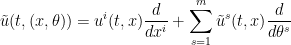
for some “swirl” fields ![{\tilde u^s: [0,T] \times M \rightarrow {\bf R}}](https://s0.wp.com/latex.php?latex=%7B%5Ctilde+u%5Es%3A+%5B0%2CT%5D+%5Ctimes+M+%5Crightarrow+%7B%5Cbf+R%7D%7D&bg=ffffff&fg=000000&s=0&c=20201002)


The base component
of this flow is then a flow on the two-dimensional 

On a fixed 


Theorem 1
- (i) (Generic inextendibility) Assume
. Then
is of the first category in
- (ii) (Non-rigidity) Assume
(with an arbitrary metric
More informally, starting with an incompressible flow
These results fall short of my hopes to use the ability to extend the manifold to create universal behaviour in Euler flows, because of the fact that each flow requires a different extension in order to achieve the desired dynamics. Still it does seem to provide a little bit of support to the idea that high-dimensional Euler flows are quite “flexible” in their behaviour, though not completely so due to the generic inextendibility phenomenon. This flexibility reminds me a little bit of the flexibility of weak solutions to equations such as the Euler equations provided by the “
The proof of part (i) of the theorem basically proceeds by a dimension counting argument (similar to that in the proof of Proposition 9 of these recent lecture notes of mine). Heuristically, the point is that an arbitrary incompressible flow 


The proof of part (ii) proceeds by direct calculation of the effect of the warping factors and swirl velocities, which effectively create a forcing term (of Boussinesq type) in the first equation of (1) that is a combination of functions of the Eulerian spatial coordinates 

We consider the incompressible Euler equations on the (Eulerian) torus 


As noted previously, the kinetic energy
 is the Euclidean metric. Indeed, if one assumes that are continuously differentiable in both space and time on
 ![{[0,T] \times \mathbf{T}}](https://s0.wp.com/latex.php?latex=%7B%5B0%2CT%5D+%5Ctimes+%5Cmathbf%7BT%7D%7D&bg=ffffff&fg=000000&s=0&c=20201002) , then one can multiply the equation (1) by
, then one can multiply the equation (1) by  and contract against
  to obtain
![{[0,T] \times \mathbf{T}_E}](https://s0.wp.com/latex.php?latex=%7B%5B0%2CT%5D+%5Ctimes+%5Cmathbf%7BT%7D_E%7D&bg=ffffff&fg=000000&s=0&c=20201002) and uses Stokes’ theorem, one obtains the required energy conservation law
and uses Stokes’ theorem, one obtains the required energy conservation law 
 is not a test function and so one cannot immediately integrate (1) against . And indeed, as we shall soon see, it is now known that once the regularity of is low enough, energy can “escape to frequency infinity”, leading to failure of the energy conservation law, a phenomenon known in physics as anomalous energy dissipation.
But what is the precise level of regularity needed in order to for this anomalous energy dissipation to occur? To make this question precise, we need a quantitative notion of regularity. One such measure is given by the Hölder space 


 lies between the space
  of continuous functions and the space
  of continuously differentiable functions, and informally describes a space of functions that is “
 times differentiable” in some sense. The above derivation of the energy conservation law involved the integral
 once
once  . More precisely, one can make
Conjecture 1 (Onsager’s conjecture) Let, and let
.
- (i) If
to the Euler equations (in the Leray form
) obeys the energy conservation law (3).
- (ii) If
, then there exist weak solutions
This conjecture was originally arrived at by Onsager by a somewhat different heuristic derivation; see Remark 7. The numerology is also compatible with that arising from the Kolmogorov theory of turbulence (discussed in this previous post), but we will not discuss this interesting connection further here.
The positive part (i) of Onsager conjecture was established by Constantin, E, and Titi, building upon earlier partial results by Eyink; the proof is a relatively straightforward application of Littlewood-Paley theory, and they were also able to work in larger function spaces than 


In these notes we will first establish (i), then discuss the convex integration method in the original context of the Nash-Kuiper embedding theorem. Before tackling the Onsager conjecture (ii) directly, we discuss a related construction of high-dimensional weak solutions in the Sobolev space 
We thank Phil Isett for some comments and corrections.

Recent Comments